Trilateration and Multilateration
Nostalgia can be bittersweet, as it reminds you that time moves forward. While digging through my undergraduate documents, I was reminded of my old Bachelor project on Multilateration/Trilateration.
Multilateration is the process of determining the location of an object from range measurements to several nodes at known locations. By a node, I mean any device capable of transmitting or receiving a signal from which a distance can be measured. To me, this is an interesting geometry problem, where the ranges are usually obtained through RF signals. You can find the concept applied indoors, e.g., with ultra-wideband (UWB) or WiFi signals, as well as outdoors, with GPS being the most famous example. As for the naming, I will stick with the term Multilateration, as it implies using as many nodes as required, whereas Trilateration often refers to using exactly three range values. Honestly, people use these terms interchangeably.
In this post, I want to cover the basics of computing the position when the ranges are given. The math is simpler than you might expect, as most of the heavy lifting is done by basic linear algebra. I will also briefly discuss how the ranges themselves are measured in the first place, as this is where most errors in practice come from. At the end of the post, you will find a Python implementation of the equations mentioned here.
Computing Position from Ranges in 3D
Some quick terminology first: I will call the fixed nodes with known locations anchors, and the node with the unknown location we want to determine the tag.
As mentioned earlier, the word “Trilateration” often refers to having only three range measurements, while using more sensors establishes an overdetermined solution. The image below shows the range sphere of every anchor relative to the tag whose location we are trying to find. Obviously, each anchor relative to the tag has infinite possible solutions for the tag’s location, which form a sphere. Every time another measurement is captured at a different location, the solution from one anchor intersects with another, reducing the degrees of freedom. In the case of three anchors, this reduces the degrees of freedom to two possible solutions. When using one additional sensor, we only have one solution. Of course, how the sensors are located impacts the quality of the solution when there is uncertainty in the range measurements, e.g., due to noise or multipath reflections.
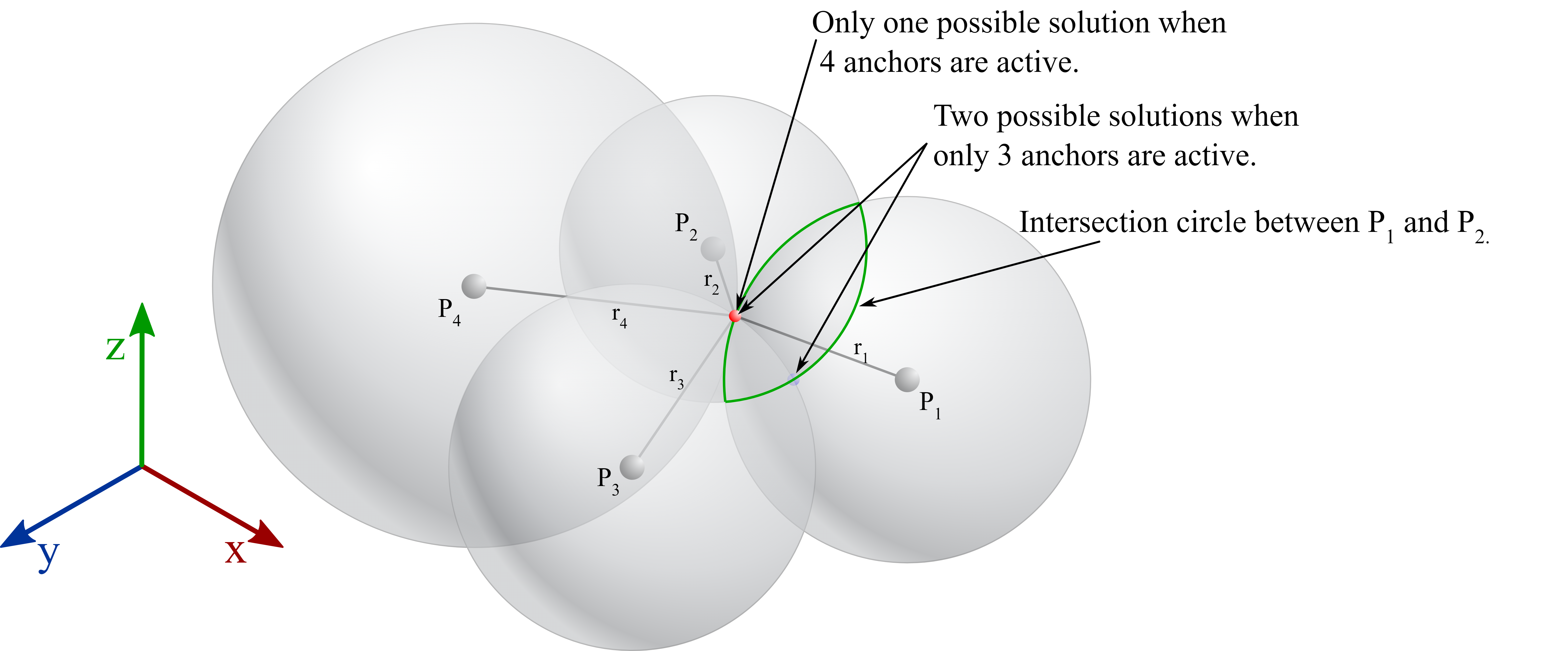 Fig. 1.: The general problem of multilateration in 3D space.
There are several ways to compute the tag location from range measurements. I will discuss two methods: the first is the direct method using linear least squares while complying with the constraints. The second is non-linear optimization, where I will use Newton’s method and also mention how it relates to the often-used Gauss-Newton method. For a general overview of the topic, the Wikipedia pages on Trilateration and True-range multilateration are a good start.
Direct Method
Each anchor is located at a known position $\bs{p}_i = [x_i,\ y_i,\ z_i]^T$ and delivers a measured range $r_i$ to the tag at the unknown location $\bs{p} = [x,\ y,\ z]^T$. Every range measurement is literally the equation of a sphere centered at the corresponding anchor:
\[(x_i - x)^2 + (y_i - y)^2 + (z_i - z)^2 = r_i^2, \qquad i = 1,2,\ldots,N \label{eq:1}\]This is a non-linear system of equations in the unknowns (i.e., $\bs{p} = [x,\ y,\ z]^T$). However, if we expand the squared brackets and rearrange the terms, something nice happens:
\[\underbrace{x^2 + y^2 + z^2}_{\|\bs{p}\|^2} - 2x_ix - 2y_iy - 2z_iz = r_i^2 - \underbrace{(x_i^2 + y_i^2 + z_i^2)}_{\|\bs{p}_i\|^2} \label{eq:2}\]The only non-linear term left is $x^2 + y^2 + z^2$, and it is the same in every equation. So, we simply declare it as an additional unknown [1]. Collecting all $N$ equations in matrix notation gives:
\[\underbrace{\begin{bmatrix} 1 & -2x_1 & -2y_1 & -2z_1\\ 1 & -2x_2 & -2y_2 & -2z_2\\ \vdots & \vdots & \vdots & \vdots\\ 1 & -2x_N & -2y_N & -2z_N \end{bmatrix}}_{\bs{A}} \underbrace{\begin{bmatrix} x^2 + y^2 + z^2\\ x\\ y\\ z \end{bmatrix}}_{\bs{x}} = \underbrace{\begin{bmatrix} r_1^2 - \|\bs{p}_1\|^2\\ r_2^2 - \|\bs{p}_2\|^2\\ \vdots\\ r_N^2 - \|\bs{p}_N\|^2 \end{bmatrix}}_{\bs{b}} \label{eq:3}\]where $\lVert\bs{p}_N\rVert^2 = x_N^2 + y_N^2 + z_N^2$. Of course, we didn’t get this linearity for free. The four unknowns are not independent of each other, as the first element is coupled to the remaining three through a quadratic constraint:
\[\bs{A}\bs{x} = \bs{b}, \qquad \bs{x} = [x_0,\ x_1,\ x_2,\ x_3]^T, \qquad x_0 = x_1^2 + x_2^2 + x_3^2 \label{eq:4}\]What I like about this formulation is that the matrix $\bs{A}$ depends only on the anchor locations. Therefore, the rank of $\bs{A}$ is purely a statement about the anchor geometry, and it tells us everything about the solvability of the problem. Depending on how the anchors are arranged, the problem falls into one of three geometric situations. I go through all three below, and then a general method that enforces the constraint for all of them at once.
Anchors spanning 3D space (unique solution)
This requires at least four anchors that do not all lie in a common plane. In this case $\bs{A}$ has full column rank, i.e., $\mathrm{rank}(\bs{A}) = 4$, and we don’t even need the constraint in Equation \eqref{eq:4}. The solution is directly given by least squares:
\[\hat{\bs{x}} = (\bs{A}^T\bs{A})^{-1}\bs{A}^T\bs{b} \label{eq:5}\]The estimated position is given by the last three elements of $\hat{\bs{x}}$. The first element is an estimate of $x^2+y^2+z^2$, which you get for free and can use as a plausibility check of the solution. Naturally, using more than four anchors makes the system overdetermined and the least squares solution averages out the errors in the ranges.
Anchors confined to a plane (two solutions)
This is what you get with exactly three anchors that don’t lie on one line (three points always define a plane), but it also happens with any number of anchors that were unluckily installed in a common plane. Here $\mathrm{rank}(\bs{A}) = 3$ and the null space of $\bs{A}$ has dimension one. Hence, the general solution is written as:
\[\bs{x} = \bs{x}_\mathrm{p} + t\,\bs{x}_\mathrm{h} \label{eq:6}\]where $\bs{x}_\mathrm{p}$ is a particular solution (e.g., the minimum-norm solution via the pseudo-inverse), $\bs{x}_\mathrm{h}$ is the homogeneous solution satisfying $\bs{A}\bs{x}_\mathrm{h} = \bs{0}$, and $t$ is an unknown scalar. This is where the constraint from Equation \eqref{eq:4} comes to the rescue. To keep the notation compact, I split both vectors into their first element and the remaining three elements, i.e., $\bs{x}_\mathrm{p} = [x_{0\mathrm{p}},\ \bs{u}^T]^T$ and $\bs{x}_\mathrm{h} = [x_{0\mathrm{h}},\ \bs{v}^T]^T$. Substituting Equation \eqref{eq:6} into the constraint results in:
\[x_{0\mathrm{p}} + t\,x_{0\mathrm{h}} = \|\bs{u} + t\,\bs{v}\|^2 \label{eq:7}\]which, after expanding the squared norm and collecting the coefficients of $t$, is just a quadratic equation:
\[t^2\underbrace{\|\bs{v}\|^2}_{a} + t\,\Big(\underbrace{2\bs{u}^T\bs{v} - x_{0\mathrm{h}}}_{b}\Big) + \underbrace{\|\bs{u}\|^2 - x_{0\mathrm{p}}}_{c} = 0 \label{eq:8}\]solved by the good old quadratic formula:
\[t_{1,2} = \frac{-b\pm\sqrt{b^2 - 4ac}}{2a} \quad\Longrightarrow\quad \bs{x} = \bs{x}_\mathrm{p} + t_{1,2}\,\bs{x}_\mathrm{h} \label{eq:9}\]So we end up with two solutions, and these are exactly the two candidate points illustrated in Fig. 1. Geometrically, the two solutions are mirror images of each other about the plane spanned by the anchors. This is quite intuitive: the anchors cannot distinguish between above and below their own plane. In practice, you resolve the ambiguity with prior knowledge, e.g., if all anchors are mounted at the ceiling, the tag is below them. One more practical detail from [1]: when the ranges contain errors, the discriminant $b^2 - 4ac$ can become negative and $t_{1,2}$ come as a complex conjugate pair. In that case, taking the real part of the solutions is the best estimate you can get.
Anchors on a line (no unique solution)
Now $\mathrm{rank}(\bs{A}) = 2$ and the null space has dimension two, i.e., two unknown scalars, but we still have only one constraint. Therefore, there are infinitely many solutions. This is also geometrically obvious: spheres centered on a common axis intersect in circles, and every point on that circle is a valid answer. No math can rescue this case, so don’t place your anchors on a line 😉. In fact, even being close to degenerate geometry makes $\bs{A}$ ill-conditioned and amplifies the range errors. The navigation folks have a name for this error amplification: dilution of precision.
Enforcing the constraint via the SVD
You might have noticed that for $\mathrm{rank}(\bs{A}) = 4$, I simply ignored the constraint. Nothing stops us from enforcing it there as well, and the tool for that is the singular value decomposition (SVD). The SVD factors our matrix as
\[\bs{A} = \bs{U}\bs{\Sigma}\bs{V}^T, \qquad \bs{V} = [\bs{v}_1,\ \bs{v}_2,\ \bs{v}_3,\ \bs{v}_4], \qquad \sigma_1 \geq \sigma_2 \geq \sigma_3 \geq \sigma_4 \geq 0 \label{eq:10}\]where the columns of $\bs{V}$ are the right singular vectors, sorted by their singular values $\sigma_k$. What we are after is the last column $\bs{v}_4$, the direction belonging to the smallest singular value $\sigma_4$. A full-rank matrix has no null space, but $\bs{v}_4$ is the next best thing: it is the direction along which $\bs{A}$ acts the weakest, so nudging the solution along it disturbs the least squares fit the least (the residual only grows by $\sigma_4^2 t^2$). We therefore set $\bs{x}_\mathrm{h} = \bs{v}_4$ and reuse the exact same machinery as the planar case. In short, the recipe is:
- Compute the least squares solution $\bs{x}_\mathrm{p}$ from Equation \eqref{eq:5}.
- Take $\bs{x}_\mathrm{h} = \bs{v}_4$ from the SVD of $\bs{A}$.
- Plug $\bs{x} = \bs{x}_\mathrm{p} + t\,\bs{x}_\mathrm{h}$ into the constraint and solve the quadratic in Equation \eqref{eq:8} for $t$.
- Of the two roots, keep the one that leads to a solution closest to a known estimate (e.g., $\bs{x}_\mathrm{p}$ if the problem is determined or overdetermined).
There is a nice sanity check hidden in the last step. If the ranges are exact, the least squares solution already satisfies the constraint, so $c = 0$ in Equation \eqref{eq:8}. The quadratic then factors as $t(a\,t + b) = 0$ with roots $t = 0$ and $t = -b/a$, and $t = 0$ is the answer, i.e., no correction needed. Once the ranges carry errors, $t$ drifts away from zero and applies the smallest nudge that makes the constraint hold exactly. The same recipe also handles the planar (rank 3) case for free, since there $\sigma_4 = 0$, so $\bs{v}_4$ is the genuine null space vector and the two roots become the two mirror solutions rather than a small correction. This is why the direct_method function in the Python code below is written as one general routine, toggled by its force_constraint argument.
2D case: everything above carries over to 2D by deleting the $z$ column in $\bs{A}$ and the $z$ terms in the unknowns. Then you need at least three anchors not on a line for a unique solution, while two anchors deliver two solutions mirrored about the line connecting the anchors.
Non-linear Optimization
The direct method takes the range values at face value, i.e., it looks for the point where all spheres truly intersect. With measurement errors, such a point generally doesn’t exist, and only when the system is overdetermined does it provide a best estimate. A more natural way to think about the problem is to define for each anchor a residual error that describes how much the distance to a candidate position disagrees with the measured range:
\[f_i(\bs{p}) = \|\bs{p}_i - \bs{p}\| - r_i \label{eq:11}\]and then find the position that minimizes the sum of squared residuals:
\[F(\bs{p}) = \frac{1}{2}\sum_{i=1}^{N}f_i^2(\bs{p}) \label{eq:12}\]where $N\geq 3$, i.e., it can also handle the overdetermined case. This is a classic non-linear least squares problem, and there is no closed-form solution. So we iterate over a linearized version of the problem. Methods such as Newton’s method let us approximate the objective function around the current estimate $\bs{p}_k$ with its second-order Taylor expansion:
\[F(\bs{p}) \approx F(\bs{p}_k) + \bs{g}_k^T(\bs{p} - \bs{p}_k) + \frac{1}{2}(\bs{p} - \bs{p}_k)^T\bs{H}_k(\bs{p} - \bs{p}_k) \label{eq:13}\]where $\bs{g}_k$ and $\bs{H}_k$ are the gradient and Hessian of $F(\bs{p})$ evaluated at $\bs{p}_k$. Minimizing the right-hand side of Equation \eqref{eq:13} with respect to $\bs{p}$ gives the well-known Newton update:
\[\bs{p}_{k+1} = \bs{p}_k - \bs{H}_k^{-1}\bs{g}_k \label{eq:14}\]So, all we need are the gradient and Hessian in closed form. The only derivative rule required beyond the standard chain and product rules is the gradient of the Euclidean distance:
\[\nabla f_i(\bs{p}) = \nabla\|\bs{p}_i - \bs{p}\| = -\frac{\bs{p}_i - \bs{p}}{\|\bs{p}_i - \bs{p}\|} \label{eq:15}\]Applying the chain rule to Equation \eqref{eq:12} delivers the gradient:
\[\bs{g}(\bs{p}) = \nabla F(\bs{p}) = \sum_{i=1}^{N}\frac{r_i - \|\bs{p}_i - \bs{p}\|}{\|\bs{p}_i - \bs{p}\|}\left(\bs{p}_i - \bs{p}\right) \label{eq:16}\]and differentiating once more with the product rule delivers the Hessian:
\[\bs{H}(\bs{p}) = \sum_{i=1}^{N}\left[\frac{r_i}{\|\bs{p}_i - \bs{p}\|^3}(\bs{p}_i - \bs{p})(\bs{p}_i - \bs{p})^T + \left(1 - \frac{r_i}{\|\bs{p}_i - \bs{p}\|}\right)\bs{I}\right] \label{eq:17}\]I prefer this outer-product form since it translates directly into code. If you multiply everything out, you get the familiar $3\times 3$ matrix of second-order partial derivatives $\partial^2 F/\partial x^2$, $\partial^2 F/\partial x\partial y$, and so on.
Two remarks worth making here. First, notice that both the gradient and Hessian divide by $\lVert\bs{p}_i - \bs{p}\rVert$. That means the objective function is not differentiable at the anchor locations themselves, and Newton’s method needs a starting point. The obvious choice is to initialize with the solution of the direct method, after which a handful of iterations is typically enough.
Second, Newton’s method with the exact Hessian is not the only option. If we stack the residuals into a vector $\bs{f} = [f_1,\ f_2,\ \ldots,\ f_N]^T$, its Jacobian $\bs{J}_{\bs{f}}$ is an $N\times 3$ matrix whose $i$-th row is $-(\bs{p}_i - \bs{p})^T/\lVert\bs{p}_i - \bs{p}\rVert$, and the gradient and Hessian can be written as:
\[\bs{g} = \bs{J}_{\bs{f}}^T\bs{f}, \qquad \bs{H} = \bs{J}_{\bs{f}}^T\bs{J}_{\bs{f}} + \sum_{i=1}^{N}f_i(\bs{p})\nabla^2 f_i(\bs{p}) \label{eq:18}\]The Gauss-Newton method keeps only the term $\bs{J}_{\bs{f}}^T\bs{J}_{\bs{f}}$ and drops the second-order term, which is justified when the residuals are small, i.e., when the ranges are reasonably accurate. Adding damping to that leads to the Levenberg-Marquardt method, which is what most software implementations of non-linear least squares actually use, e.g., SciPy’s least_squares. For our small problem with only three unknowns, the exact Hessian is cheap anyway, so we might as well use it.
Methods for Range Estimation
Until now, I treated the ranges $r_i$ as given. In practice, measuring them is the actual hard part. The most common approach in RF systems is time-based ranging, where the distance follows from the time of flight $\tau_F$ of a transmitted signal:
\[d = v\,\tau_F \label{eq:19}\]where $v$ is the propagation speed, which in air is basically the speed of light $c_0\approx 3\times10^8\,\mathrm{m/s}$. To appreciate the challenge here: light travels about $30\,\mathrm{cm}$ in one nanosecond. So, every nanosecond of timing error translates to $30\,\mathrm{cm}$ of range error.
The simplest scheme is one-way time of arrival (TOA): node A transmits a packet at time $t_1$ and node B receives it at time $t_2$, as illustrated below.
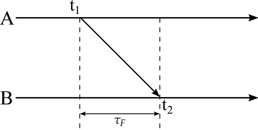 Fig. 2.: One-way TOA ranging.
The distance is then computed as:
\[\tau_F = t_2 - t_1 \quad\Longrightarrow\quad d = c_0(t_2 - t_1) \label{eq:20}\]The catch is that $t_1$ and $t_2$ are read from two different clocks, so this only works if both nodes are synchronized to a common time reference. Keeping two independent RF nodes synchronized at sub-nanosecond level is difficult and expensive.
The way around synchronization is two-way TOA, where we measure the round-trip time instead. Node A transmits at $t_1$, node B replies after a known response delay $\tau_d$, and node A receives the reply at $t_2$. Both timestamps now come from the same clock in node A.
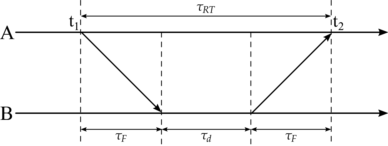 Fig. 3.: Two-way TOA ranging.
The round-trip time contains the time of flight twice plus the response delay:
\[\tau_{RT} = t_2 - t_1 = 2\tau_F + \tau_d \quad\Longrightarrow\quad d = c_0\left(\frac{t_2 - t_1 - \tau_d}{2}\right) \label{eq:21}\]This is not entirely free of clock problems either. Node B measures its response delay $\tau_d$ with its own clock, so any relative frequency offset between the two clocks accumulates an error over the duration of $\tau_d$. There are refined protocols to suppress this effect (e.g., double-sided two-way ranging), but the principle stays the same. For a much deeper treatment of time-based ranging and its error sources, especially multipath propagation, see [2] and [3].
For completeness, I should mention another related scheme. In time difference of arrival (TDOA), only the anchors need to be synchronized, while the tag just transmits. Each pair of anchors then measures a difference of arrival times, which constrains the tag to a hyperboloid instead of a sphere, and the math changes accordingly; see the Wikipedia page on Multilateration. Lastly, you might wonder where ultra-wideband (UWB) fits in all of this. The time resolution of a pulse is inversely proportional to its bandwidth, so with at least $500\,\mathrm{MHz}$ of bandwidth, UWB signals deliver sub-nanosecond pulses. That is what makes centimeter-level ranging possible in the first place, and it also helps to resolve multipath reflections that would smear out the timing estimate of narrowband signals [2].
Python Code
Below is a self-contained implementation of both methods using plain NumPy. The function direct_method() implements Equations \eqref{eq:3}-\eqref{eq:10}, including the rank handling and the optional force_constraint toggle, and newton_method() implements Equations \eqref{eq:14}, \eqref{eq:16}, and \eqref{eq:17}. The example places four anchors, simulates ranges with some noise, and estimates the position with both methods.
1
2
3
4
5
6
7
8
9
10
11
12
13
14
15
16
17
18
19
20
21
22
23
24
25
26
27
28
29
30
31
32
33
34
35
36
37
38
39
40
41
42
43
44
45
46
47
48
49
50
51
52
53
54
55
56
57
58
59
60
61
62
63
64
65
66
67
68
69
70
71
72
73
74
75
76
77
78
79
80
81
82
83
84
85
86
87
88
89
90
91
92
93
94
95
96
97
98
99
100
101
102
103
104
105
106
107
108
109
110
111
import numpy as np

def direct_method(anchors, ranges, force_constraint=False, tol=1e-6):
    """
    Estimate the tag position by solving the linearized system A@x = b.

    Parameters
    ----------
    anchors : (N, 3) or (N, 2) array of anchor locations.
    ranges : length-N array of measured ranges to the tag.
    force_constraint : if True, always enforce the constraint via the SVD.
    tol : relative threshold on the smallest singular value of A below which
          the anchor geometry is treated as degenerate.

    Returns
    -------
    A single position, or two mirrored candidates when the geometry is degenerate.
    """
    anchors = np.atleast_2d(anchors)
    ranges  = np.asarray(ranges)

    A = np.hstack([np.ones((len(anchors), 1)), -2*anchors])
    b = ranges**2 - np.sum(anchors**2, axis=1)

    xp = np.linalg.pinv(A)@b            # particular solution (least squares)
    s, Vt = np.linalg.svd(A)[1:]        # singular values and right vectors
    xh = Vt[-1]                         # weakest right singular direction

    # degenerate geometry: fewer equations than unknowns, or A ill-conditioned
    degenerate = len(s) < A.shape[1] or s[-1] < tol*s[0]

    if not degenerate and not force_constraint:
        return xp[1:]  # constraint is redundant, least squares is enough

    # enforce the constraint x0 = x1^2 + x2^2 + x3^2 to solve for t
    a = xh[1:]@xh[1:]
    b = 2*xp[1:]@xh[1:] - xh[0]
    c = xp[1:]@xp[1:] - xp[0]
    t = np.roots([a, b, c]).real       # take real part if ranges have errors

    if not degenerate:
        t = t[np.argmin(np.abs(t))]    # smaller correction, other root is spurious
        return xp[1:] + t*xh[1:]

    # degenerate: the two roots are the mirrored candidate solutions
    return np.array([xp[1:] + t[0]*xh[1:], xp[1:] + t[1]*xh[1:]])

def newton_method(anchors, ranges, p0, max_iter=50, tol=1e-10):
    """
    Refine a position estimate by minimizing the sum of squared range errors.

    Parameters
    ----------
    anchors : (N, 3) or (N, 2) array of anchor locations.
    ranges : length-N array of measured ranges to the tag.
    p0 : initial position estimate.
    max_iter : maximum number of iterations.
    tol : stop when the Newton step is smaller than this.

    Returns
    -------
    The estimated position.
    """
    anchors = np.atleast_2d(anchors)
    ranges  = np.asarray(ranges)
    p = np.asarray(p0, dtype=float)

    for _ in range(max_iter):
        d = anchors - p                    # rows are (p_i - p)
        dist = np.linalg.norm(d, axis=1)   # ||p_i - p||
        # gradient and Hessian evaluated at current position
        g = d.T@((ranges - dist)/dist)
        H = (d.T*(ranges/dist**3))@d + np.sum(1 - ranges/dist)*np.eye(len(p))
        # newton update
        step = np.linalg.solve(H, g)
        p = p - step
        if np.linalg.norm(step) < tol:
            break
    return p

if __name__ == '__main__':
    rng = np.random.default_rng(42)

    anchors = np.array([[0.0, 0.0, 0.0],
                        [6.0, 1.0, 0.5],
                        [1.0, 5.0, 0.0],
                        [3.0, 2.0, 4.0]])
    p_true = np.array([2.2, 3.1, 1.4])

    # simulate measured ranges with some noise
    ranges = np.linalg.norm(anchors - p_true, axis=1) + 0.05*rng.standard_normal(len(anchors))

    print('True position:     ', p_true)

    # three anchors --> two candidate solutions
    p_direct3 = direct_method(anchors[:3], ranges[:3])
    print('Direct (3 anchors):', p_direct3[0], ' or ', p_direct3[1])

    # four anchors --> unique least squares solution
    p_direct4 = direct_method(anchors, ranges)
    print('Direct (4 anchors):', p_direct4)

    # same, but forcing the quadratic constraint via the SVD
    p_forced = direct_method(anchors, ranges, force_constraint=True)
    print('Direct (forced):   ', p_forced)

    # refine with Newton's method using the direct solution as starting point
    p_newton = newton_method(anchors, ranges, p_direct4)
    print('Newton (4 anchors):', p_newton)

    # EOF
Running the script gives the following output:
1
2
3
4
5
True position:      [2.2 3.1 1.4]
Direct (3 anchors): [ 2.46709275  3.03893848 -1.10089829]  or  [2.25131509 3.08209401 1.40212254]
Direct (4 anchors): [2.25597006 3.08116302 1.34812483]
Direct (forced):    [2.16228553 2.95767037 1.30288335]
Newton (4 anchors): [2.2597113  3.08958294 1.34988443]
You can see everything discussed earlier in action: with three anchors we get two candidates, where one is close to the true position and the other is its mirror image about the plane of the three anchors. With four well-placed anchors, the solution is unique, and forcing the constraint or refining with Newton’s method both nudge it a little closer.
There is more to explore beyond this post. For example, when tracking a moving tag, solving each time instant independently gives jumpy trajectories, and combining the position solution with a motion model via a Kalman filter makes a big difference (see [4]).
References
[1] A. Norrdine, “An algebraic solution to the multilateration problem,” in Proceedings of the 3rd international conference on indoor positioning and indoor navigation (IPIN), Sydney, Australia, Nov. 2012, doi: 10.13140/RG.2.1.1681.3602.
[2] Z. Sahinoglu, S. Gezici, and I. Güvenc, Ultra-Wideband Positioning Systems: Theoretical Limits, Ranging Algorithms, and Protocols. Cambridge: Cambridge University Press, 2008, doi: 10.1017/CBO9780511541056.
[3] D. Dardari, A. Conti, U. Ferner, A. Giorgetti and M. Z. Win, “Ranging With Ultrawide Bandwidth Signals in Multipath Environments,” in Proceedings of the IEEE, vol. 97, no. 2, pp. 404-426, Feb. 2009, doi: 10.1109/JPROC.2008.2008846.
[4] G. Strang and K. Borre, Linear Algebra, Geodesy, and GPS. Wellesley, MA: Wellesley-Cambridge Press, 1997. ISBN: 9780961408862.