Multiline TRL Calibration

I believe there is a defining moment for those of us who perform RF measurements: the time before mastering TRL calibration and the time after. TRL calibration is a powerful tool for VNA calibration. More importantly for planar circuit measurements where in-situ probing is often not possible. However, as I discussed in my previous post on TRL, TRL calibration is bandwidth-limited. This is where the multiline version comes in, which enables broader frequency coverage.

The purpose of this post is to provide the mathematical background for implementing multiline TRL calibration. I will not be discussing how to implement the NIST version [1,2]; instead, I will show you my own version [3], which is based on a different formulation and makes fewer assumptions. You can check out my GitHub repository for Python scripts and measurements, where I also provide an example analyzing the statistical difference between my method and NIST’s method: https://github.com/ZiadHatab/multiline-trl-calibration

The Bandwidth Limitation of TRL Calibration

It is a good refresher to understand why TRL calibration is bandwidth-limited. To begin the discussion, we use the error box model of a two-port VNA, depicted in the diagram below. We can express this model in terms of T-parameters as follows:

\[\bs{M}_\mathrm{std} = \underbrace{k_ak_b}_{k}\underbrace{\left[\begin{matrix}a_{11} & a_{12}\\a_{21} & 1\end{matrix}\right]}_{\bs{A}}\bs{T}_\mathrm{std} \underbrace{\left[\begin{matrix}b_{11} & b_{12}\\b_{21} & 1\end{matrix}\right]}_{\bs{B}} \label{eq:1}\]

where $\bs{A}$ and $\bs{B}$ are the single port error boxes, and $k$ is the transmission error. $\bs{M}_\mathrm{std}$ and $\bs{T}_\mathrm{std}$ are the measured and actual T-parameters of the standard.

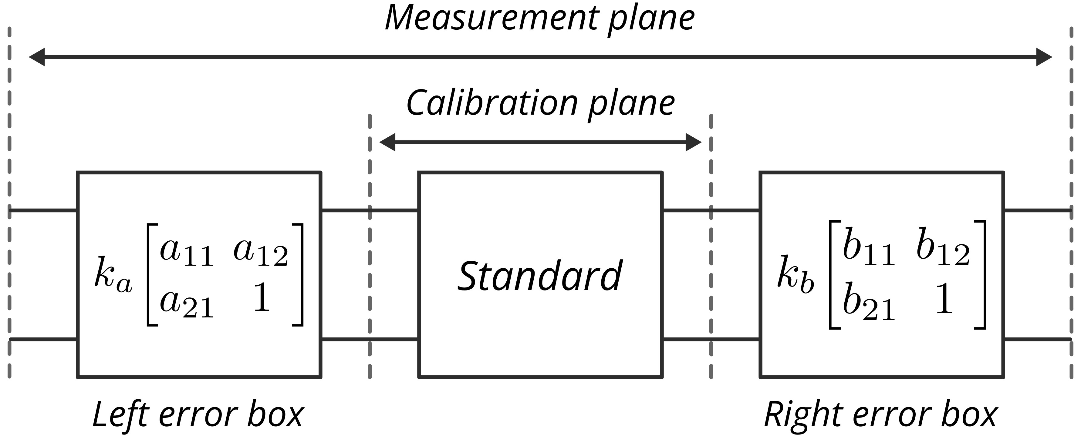Fig. 1. Two-port VNA error box model.

If we consider a matched line standard, we replace $\bs{T}_\mathrm{std}$ with a diagonal matrix describing the line as follows:

\[\bs{M}_i = k\bs{A}\underbrace{\begin{bmatrix} e^{-\gamma l_i} & 0\\ 0 & e^{\gamma l_i} \end{bmatrix}}_{\bs{L}_i}\bs{B} \label{eq:2}\]

where $l_i$ represents the length of the i-th considered line and $\gamma$ represents the propagation constant of the transmission line. The general procedure involves taking two lines with different lengths, resulting in a $2\times2$ eigenvalue problem when one measurement is multiplied by the inverse of another. This can be expressed as follows:

\[\bs{M}_i\bs{M}_j^{-1} = \bs{A}\begin{bmatrix} e^{-\gamma (l_i-l_j)} & 0\\ 0 & e^{\gamma (l_i-l_j)} \end{bmatrix}\bs{A}^{-1} \label{eq:3}\]

The same eigenvalue problem can be formulated with respect to $\bs{B}$. Regardless of the choice of the error box, when using only two lines, we face a problem given the values of the eigenvalues, i.e., $e^{\pm\gamma (l_i-l_j)}$. In the lossless or low-loss cases, $\gamma \approx j\beta$, and as $\beta$ is frequency-dependent, it is possible for the product $\beta (l_i-l_j)$ to be a multiple of $\pi$. This will result in $e^{jn\pi} = \pm 1$. If we substitute the values of $\pm1$ in the eigenvalue problem, we get:

\[\bs{M}_i\bs{M}_j^{-1} = \bs{A}\begin{bmatrix} \pm 1 & 0\\ 0 & \pm 1 \end{bmatrix}\bs{A}^{-1} = \pm\bs{I}_{2\times2} \label{eq:4}\]

Therefore, at critical frequencies, which are multiples of half-wavelength, we lose all information about the error boxes.

The frequency limitation of the TRL method can be overcome by using the multiline TRL method developed by NIST [1,2]. This method employs multiple lines of different lengths to create multiple eigenvalue problems from different line pairs. The algorithm is based on a first-order approximation of the error box to describe any statistical error as having a linear effect. By solving the eigenevalue problem of each pair, it then combines the results of the pairs linearly using the Gauss-Markov weighted linear least squares method. However, a common line to all pairs must be chosen, resulting in $N-1$ pairs for $N$ lines. The choice of the common line can be different at each frequency, often resulting in abnormal discontinuities along the frequency axis. This can also lead to poor results if one or more pairs are singular. Additionally, the method assumes equal disturbance at both ports, which may not always be the case. The multiline TRL method from NIST is optimal only when all its assumptions are met, but poor results may occur if these conditions are not met.

As mentioned earlier, I will not delve into the implementation of the NIST multiline TRL method. If you are interested in the NIST approach, please refer to [1,2]. Instead, I will present an alternative method [3] that is more reliable, does not make any approximation assumptions, and is easier to implement. I will refer to this method as the TUG multiline TRL to differentiate it from the NIST multiline TRL. TUG stands for TU Graz, the university where I conducted research on this topic. Below is a brief comparison between NIST and TUG multiline TRL methods:

NIST multiline TRL [1,2]:

• The measurement assumes a first-order approximation with respect to any disturbance, and this should also hold true in the eigenvectors of the line pairs.
• If the first-order approximation assumption holds true, multiple eigenvalue problems can be solved and combined using the Gauss-Markov estimator (weighted sum) to obtain a combined solution.
• The weights are applied to the solutions (eigenvectors) and not to the measurements themselves.
• The derived covariance matrix used to weight the eigenvectors assumes that both ports exhibit the same level of statistical error.
• During the calibration procedure, a common line is selected, which can change across frequencies and often leads to abnormal discontinuities across the frequency axis.

TUG multiline TRL [3]:

• No assumptions are made about the type of statistical error found in the measurement.
• A weighting matrix is derived to optimally combine the measurements, resulting in a single 4x4 weighted eigenvalue problem.
• The weighting matrix is derived to minimize the sensitivity of the eigenvectors by maximizing the eigengap (i.e., distance between the eigenvalues).
• There is no common line. All measurements are combined at once, so all pair combinations are implicitly used.

Derivation of TUG Multiline TRL Calibration

The basic blocks of TUG multiline TRL method are shown in the flowchart below, which basically can be simplified into three points:

• Using the line measurements to formulate and solve the $4\times 4$ weighted eigenvalue problem, which also involves computing the weighting matrix.
• Solving for the propagation constant using the line measurements and the normalized error terms.
• Denormalizing the error terms that were solved through the eigendecomposition with help of thru and reflect standards.

In the original derivation of TUG multiline TRL discussed in [3], I used an optimization procedure to compute the propagation constant and weighting matrix. In [4], I updated my approach by using Takagi decomposition to compute the weighting matrix and linear least squares to compute the propagation constant.

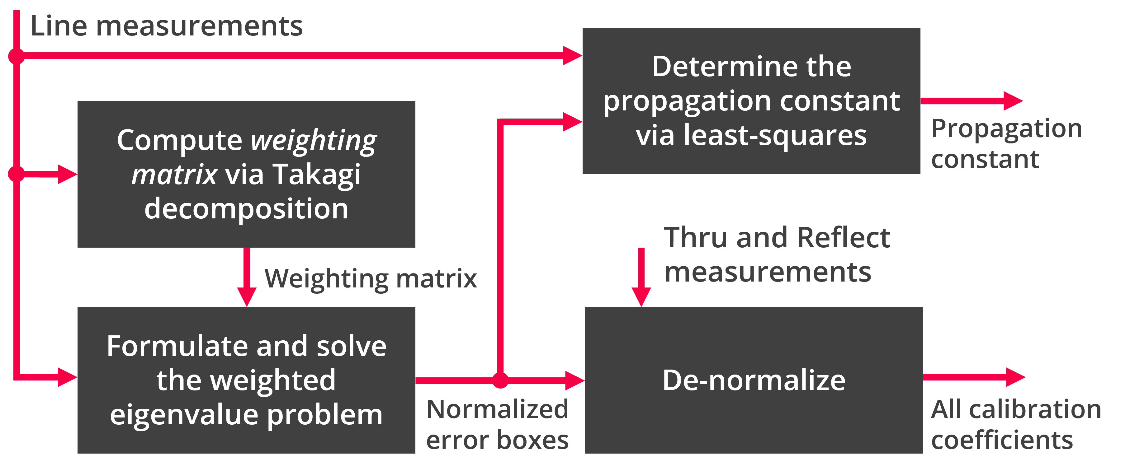Fig. 2. Flowchart diagram of the TUG Multiline TRL calibration. The line measurements include the thru measurement. If a non-zero thru measurement is used, the propagation constant is also utilized to shift the reference plane to the desired location.

Formulating the eigenvalue problem

We’ll start by using the error box model to measure a line standard, which is given for the i-th line in terms of T-parameters as follows:

\[\bs{M}_i = k\bs{A}\bs{L}_i\bs{B} \label{eq:5}\]

In the TUG multiline TRL formulation, we use Kronecker product $\otimes$ notation and apply the vectorization operator $\vc{}$ to express the above equation. When we apply vectorization to the product of three matrices, the following property generally holds:

\[\vc{\bs{X}\bs{Y}\bs{Z}} = (\bs{Z}^T\otimes \bs{X})\vc{\bs{X}} \label{eq:6}\]

To learn more about the Kronecker product and vectorization operator, you can refer to [5] or any online resources, as Wikipedia.

By applying the vectorization to the error box model above, we have the following result:

\[\vc{\bs{M}_i} = k(\bs{B}^T\otimes\bs{A})\vc{\bs{L}_i} \label{eq:7}\]

Below is the expanded evaluation of the Kronecker product so you can see what it looks like:

\[\bs{B}^T\otimes\bs{A} = \left[\begin{matrix}a_{11} b_{11} & a_{12} b_{11} & a_{11} b_{21} & a_{12} b_{21}\\a_{21} b_{11} & b_{11} & a_{21} b_{21} & b_{21}\\a_{11} b_{12} & a_{12} b_{12} & a_{11} & a_{12}\\a_{21} b_{12} & b_{12} & a_{21} & 1\end{matrix}\right] \label{eq:8}\]

We also require the inverse measurement of the line. It is defined as follows for the i-th line measurement:

\[\bs{M}_i^{-1} = \frac{1}{k}\bs{B}^{-1}\bs{L}_i^{-1}\bs{A}^{-1} \label{eq:9}\]

Similarly, by applying the vectorization operator, we obtain the following:

\[\vc{\bs{M}_i^{-1}} = \frac{1}{k}(\bs{A}^{-T}\otimes\bs{B}^{-1})\vc{\bs{L}_i^{-1}} \label{eq:10}\]

We will now use two properties of the Kronecker product:

• Transpose and inverse distribution property: $(\bs{X}\otimes\bs{Y})^{-1} = \bs{X}^{-1}\otimes\bs{Y}^{-1}$ and $(\bs{X}\otimes\bs{Y})^T = \bs{X}^T\otimes\bs{Y}^T$.
• Matrix Commutation: for a specific permutation matrix $\bs{P}$, the Kronecker product is commutative as follows: $\bs{X}\otimes\bs{Y} = \bs{P}(\bs{Y}\otimes\bs{X})\bs{P}$. The structure of $\bs{P}$ depends on the matrix size. An algorithm to generate the correct $\bs{P}$ given the size of the product can be found in [6].

Based on the two properties mentioned above, we arrive at the following result:

\[\begin{aligned} \vc{\bs{M}_i^{-1}} =& \frac{1}{k}(\bs{A}\otimes\bs{B}^T)^{-T}\vc{\bs{L}_i^{-1}}\\ =&\frac{1}{k}\bs{P}(\bs{B}^T\otimes\bs{A})^{-T}\bs{P}\vc{\bs{L}_i^{-1}} \end{aligned} \label{eq:11}\]

where $\bs{P}$ has a size of $4\times 4$ and is given as follows:

\[\bs{P} = \begin{bmatrix} 1 & 0 & 0 & 0\\ 0 & 0 & 1 & 0\\ 0 & 1 & 0 & 0\\ 0 & 0 & 0 & 1 \end{bmatrix}, \qquad \bs{P}=\bs{P}^{-1}=\bs{P}^T. \label{eq:12}\]

We currently have two equations that both describe the same line. One equation describes the measurements, while the other describes the inverse of the measurements. Our objective is to include all lines in our analysis. Since the error box resulting from the Kronecker product remains constant when measuring different standards, we can easily extend the equations by adding all vectorized measurements to them, as done below:

\[\begin{aligned} \bs{M} &= k\bs{X}\bs{L}\\ \overbar{\bs{M}} &= \frac{1}{k}\bs{P}\bs{X}^{-T}\bs{P}\overbar{\bs{L}} \end{aligned} \label{eq:13}\]

where

\[\begin{align} \bs{M} &= \begin{bmatrix} \vc{\bs{M}_1} & \vc{\bs{M}_2} & \cdots & \vc{\bs{M}_N} \end{bmatrix},\label{eq:14}\\[5pt] \bs{L} &= \begin{bmatrix} \vc{\bs{L}_1} & \vc{\bs{L}_2} & \cdots & \vc{\bs{L}_N} \end{bmatrix},\label{eq:15}\\[5pt] \bs{X} &= \bs{B}^T\otimes\bs{A},\label{eq:16}\\[5pt] \overbar{\bs{M}} &= \begin{bmatrix} \vc{\bs{M}_1^{-1}} & \vc{\bs{M}_2^{-1}} & \cdots & \vc{\bs{M}_N^{-1}} \end{bmatrix},\label{eq:17}\\[5pt] \overbar{\bs{L}} &= \begin{bmatrix} \vc{\bs{L}_1^{-1}} & \vc{\bs{L}_2^{-1}} & \cdots & \vc{\bs{L}_N^{-1}} \end{bmatrix},\label{eq:18} \end{align}\]

In [3], I simplified the equations for $\overline{\bs{M}}$ and $\overline{\bs{L}}$ by rewriting them in terms of the non-inverse version. This was done based on the relationship of a $2 \times 2$ matrix inverse when applied to it the vectorization operator.

\[\vc{\bs{M}_i^{-1}} = \bs{Q}\vc{\bs{M}_i}\frac{1}{\det\left( \bs{M}_i \right)}; \qquad \vc{\bs{L}_i^{-1}} = \bs{Q}\vc{\bs{L}_i}\underbrace{\frac{1}{\det\left( \bs{L}_i \right)}}_{=1} \label{eq:19}\]

where $\bs{Q}$ is given as follows:

\[\bs{Q} = \begin{bmatrix} 0 & 0 & 0 & 1\\ 0 & -1 & 0 & 0\\ 0 & 0 & -1 & 0\\ 1 & 0 & 0 & 0 \end{bmatrix}, \qquad \bs{Q}=\bs{Q}^{-1}=\bs{Q}^T \label{eq:20}\]

The proof of the above equations is straightforward. However, it should be noted that this is only valid for $2 \times 2$ matrices, as the adjugate matrix of this size is essentially a permutation operation with sign change. Additionally, it should be noted that $\det(\bs{L}_i) = 1$, as line standards are reciprocal devices.

With the above simplification, we can replace $\overbar{\bs{M}}$ and $\overbar{\bs{L}}$ with the following expressions:

\[\overbar{\bs{M}} = \bs{Q}\bs{M}\bs{D}^{-1}; \qquad \overbar{\bs{L}} = \bs{Q}\bs{L} \label{eq:21}\]

where

\[\bs{D} = \mathrm{diag}\left( \begin{bmatrix} \det(\bs{M}_1) & \det(\bs{M}_2) & \cdots & \det(\bs{M}_N) \end{bmatrix}\right) \label{eq:22}\]

Finally, we arrive at the following expressions:

\[\begin{aligned} \bs{M} &= k\bs{X}\bs{L}\\ \bs{Q}\bs{M}\bs{D}^{-1} &= \frac{1}{k}\bs{P}\bs{X}^{-T}\bs{P}\bs{Q}\bs{L} \end{aligned} \label{eq:23}\]

To simplify the equations further, we can apply the transpose to the second equation. This will eliminate the transpose on $\bs{X}^{-1}$. After that, we can multiply both sides by $\bs{P}$ to eliminate it on the right-hand side.

\[\begin{align} \bs{M} &= k\bs{X}\bs{L},\label{eq:24}\\[5pt] \bs{D}^{-1}\bs{M}^{T}\bs{P}\bs{Q} &= \frac{1}{k}\bs{L}^{T}\bs{P}\bs{Q}\bs{X}^{-1},\label{eq:25} \end{align}\]

with $\bs{P}\bs{Q} = \bs{Q}\bs{P}$.

We can use the two equations above to formulate the eigenvalue problem. To do this, we multiply a weighting matrix $\bs{W}$ (with dimensions $N \times N$) on the right-hand side of the first equation, and then multiply the resulting equation on the left-hand side of the second equation. The purpose of the weighting matrix will become clearer in the upcoming steps. For now, the following expression is obtained:

\[\underbrace{\bs{M}\bs{W}\bs{D}^{-1}\bs{M}^T\bs{P}\bs{Q}}_{\bs{F}:\ 4\times4} = \bs{X}\underbrace{\bs{L}\bs{W}\bs{L}^T\bs{P}\bs{Q}}_{\bs{H}:\ 4\times4}\bs{X}^{-1} \label{eq:26}\]

The expression above represents a similarity relationship between $\bs{F}$ and $\bs{H}$ through the transformation matrix $\bs{X}$. If $\bs{H}$ is diagonal, the problem can be solved through eigendecomposition. The objective is to select $\bs{W}$ in such a way that $\bs{H}$ becomes diagonal, which facilitates the computation of $\bs{X}$ through eigendecomposition (at least a normalized version).

Assuming $\bs{W}$ is any non-zero $N\times N$ matrix, we can determine its appropriate structure by expressing $\bs{H}$ in terms of $\bs{W}$ and the entries of $\bs{L}$. To begin, we consider $\bs{L}$, whose entries can be expressed by two vectors:

\[\newcommand{\horzbar}{\rule[.5ex]{2.5ex}{0.5pt}} \bs{L} = \begin{bmatrix} & \horzbar & \bs{z}^T & \horzbar & \\ & \horzbar & \bs{0} & \horzbar & \\ & \horzbar & \bs{0} & \horzbar & \\ & \horzbar & \bs{y}^T & \horzbar & \end{bmatrix} \label{eq:27}\]

where $\bs{y}$ and $\bs{z}$ are given as follows:

\[\bs{y}^T = \begin{bmatrix} e^{\gamma l_1} & e^{\gamma l_2} &\cdots & e^{\gamma l_N} \end{bmatrix},\qquad \bs{z}^T = \left[\begin{matrix} e^{-\gamma l_1} & e^{-\gamma l_2} & \cdots & e^{-\gamma l_N} \end{matrix}\right] \label{eq:28}\]

Therefore, by evaluating $\bs{H}$, we can obtain the following expression in terms of $\bs{W}$, $\bs{y}$, and $\bs{z}$:

\[\bs{H} = \begin{bmatrix} \bs{z}^T\bs{W}\bs{y} & 0 & 0 & \bs{z}^T\bs{W}\bs{z}\\ 0 & 0 & 0 & 0\\ 0 & 0 & 0 & 0\\ \bs{y}^T\bs{W}\bs{y} & 0 & 0 & \bs{y}^T\bs{W}\bs{z} \end{bmatrix} \label{eq:29}\]

To make $\bs{H}$ diagonal, we need to set the off-diagonal elements $\bs{y}^T\bs{W}\bs{y}$ and $\bs{z}^T\bs{W}\bs{z}$ to zero. This is possible since any vector-matrix product of the form $\bs{y}^T\bs{W}\bs{y}$ must be zero when $\bs{W}$ is a skew-symmetric matrix [7]. An example of a $4\times 4$ skew-symmetric matrix is given below, with its transpose property:

\[\bs{W} = \begin{bmatrix} 0 & w_{12} & w_{13} & w_{14}\\ -w_{12} & 0 & w_{23} & w_{24}\\ -w_{13} & -w_{23} & 0 & w_{34}\\ -w_{14} & -w_{24} & -w_{34} & 0 \end{bmatrix}, \qquad \bs{W} = -\bs{W}^T \label{eq:30}\]

To prove $\bs{y}^T\bs{W}\bs{y}=0$ and $\bs{z}^T\bs{W}\bs{z}=0$, when $\bs{W}$ is skew-symmetric, is simple. This is because the transpose of any scalar is equal to the scalar itself. Thus, we get:

\[\bs{y}^T\bs{W}\bs{y} = (\bs{y}^T\bs{W}\bs{y})^T = \bs{y}^T\underbrace{\bs{W}^T}_{-\bs{W}}\bs{y} = -\bs{y}^T\bs{W}\bs{y} \label{eq:31}\]

Hence, for $\bs{y}^T\bs{W}\bs{y} = -\bs{y}^T\bs{W}\bs{y}$, the solution must be equal to zero.

The matrix $\bs{H}$ will become diagonal if $\bs{W}$ has a skew-symmetric structure, regardless of its entries. We can use the skew-symmetric property of $\bs{W}$ to simplify $\bs{z}^T\bs{W}\bs{y}$ as $-\bs{y}^T\bs{W}\bs{z}$. Therefore, we can express the matrix $\bs{H}$ as follows:

\[\bs{H} = \begin{bmatrix} -\lambda & 0 & 0 & 0\\ 0 & 0 & 0 & 0\\ 0 & 0 & 0 & 0\\ 0 & 0 & 0 & \lambda \end{bmatrix}, \qquad \text{where, } \lambda = \bs{y}^T\bs{W}\bs{z} \label{eq:32}\]

We were able to convert the similarity problem into an eigenvalue problem by choosing a skew-symmetric matrix as the weighting matrix. However, we need to determine the optimal values for the entries of this matrix. We define the optimality of the weighting matrix as the matrix that minimizes the sensitivity of the eigenvectors.

According to eigendecomposition perturbation theory [8] (also on Wikipedia), the sensitivity of the eigenvectors is inversely proportional to the Euclidean distance between the eigenvalues, also known as the eigengap. Therefore, to minimize the sensitivity of the eigenvectors, we need to maximize the distance between the eigenvalues.

Since the matrix $\bs{H}$ is constructed using only the values $0$ and $\lambda$, we can maximize the distance by ensuring that $\lambda$ is as far as possible from zero. The value of $\lambda$ can be expressed in sum notation by expanding the vector-matrix product.

\[\lambda = \bs{y}^T\bs{W}\bs{z} = \sum\limits_{\begin{gathered}\\[-18pt] \scriptstyle i=1\\[-8pt]\scriptstyle i<j\leq N\end{gathered}}^{N-1}w_{ij}\left(e^{\gamma l_{ij}}-e^{-\gamma l_{ij}}\right), \qquad l_{ij} = l_i-l_j \label{eq:33}\]

To ensure that $\lambda$ is never equal to zero, we need to sum over positive values. To achieve this, we select the optimal weighting matrix $\bs{W}$ by defining its elements $w_{ij}$ as the complex conjugate of $e^{\gamma l_{ij}}-e^{-\gamma l_{ij}}$. This ensures that the sum is never zero unless all pairs have the same electrical length, which means that there is no new information from any line combinations. Therefore, $\lambda$ is given by the following equation:

\[\lambda = \bs{y}^T\bs{W}_\mathrm{opt}\bs{z} = \sum\limits_{\begin{gathered}\\[-18pt] \scriptstyle i=1\\[-8pt]\scriptstyle i<j\leq N\end{gathered}}^{N-1}\left|e^{\gamma l_{ij}}-e^{-\gamma l_{ij}}\right|^2 \label{eq:34}\]

where $\bs{W}_\mathrm{opt}$ can be shown by direct calculation to have the following form:

\[\bs{W}_\mathrm{opt} = (\bs{y}\bs{z}^T - \bs{z}\bs{y}^T)^{*} \quad\Longrightarrow\quad \bs{W}_\mathrm{opt}^H = \bs{z}\bs{y}^T - \bs{y}\bs{z}^T \label{eq:35}\]

with $()^{*}$ being the complex conjugate operator (without transpose), and $()^H$ is the Hermitian transpose (conjugate transpose).

To calculate $\bs{W}_\mathrm{opt}$, one method is to evaluate the expression above using the propagation constant and line lengths. However, at this point, we may not have an accurate estimate of the propagation constant. In the next section, I will discuss how to obtain $\bs{W}_\mathrm{opt}$ directly from the line measurements using Takagi decomposition.

Once we have $\bs{W}_\mathrm{opt}$, we need to solve for the eigenvectors that correspond to the solution of $\bs{X} = \bs{B}^{T}\otimes\bs{A}$. Eigenvectors are only unique up to a scalar multiple, so they have to be normalized to get a unique answer. Since $\bs{X}$ is a $4\times 4$ matrix, there are four eigenvectors. I chose to normalize all diagonal elements to be 1. Other normalization choices could have been made, but this choice makes it simpler to denormalize later. This results in the normalized error terms of the following form:

\[\begin{aligned} \widetilde{\bs{X}} =& \begin{bmatrix} \widetilde{\bs{x}}_1 & \widetilde{\bs{x}}_2 & \widetilde{\bs{x}}_3 & \bs{x}_4 \end{bmatrix}\\[5pt] =& \bs{X}\mathrm{diag}\left(\begin{bmatrix} a_{11}b_{11} & b_{11} & a_{11} & 1 \end{bmatrix}\right)^{-1} \\[5pt] =& \begin{bmatrix} 1 & a_{12} & b_{21} & a_{12} b_{21}\\[5pt] \frac{a_{21}}{a_{11}} & 1 & b_{21}\frac{a_{21}}{a_{11}} & b_{21}\\[5pt] \frac{b_{12}}{b_{11}} & a_{12}\frac{b_{12}}{b_{11}} & 1 & a_{12}\\[5pt] \frac{a_{21} b_{12}}{a_{11} b_{11}} & \frac{b_{12}}{b_{11}} & \frac{a_{21}}{a_{11}} & 1 \end{bmatrix} \end{aligned} \label{eq:36}\]

Many software tools can solve for eigenvectors, but we encounter an issue with eigenvectors that correspond to repeated zero eigenvalues. Since linear combinations of these eigenvectors are also eigenvectors, we have a degree of freedom to eliminate. Note that these two eigenvectors that correspond to the zero eigenvalue are referred to as the nullspace basis of the matrix.

To find the solutions for $\widetilde{\bs{x}}_2$ and $\widetilde{\bs{x}}_3$, we’ll use a linear combination of the nullspace basis of $\bs{F}$. Since $\bs{F}$ has two zero eigenvalues, it also has two nullspace bases. Here’s how we determine $\widetilde{\bs{x}}_2$ and $\widetilde{\bs{x}}_3$:

\[\begin{align} \widetilde{\bs{x}}_2 &= c_1\bs{v}^{(1)} + c_2\bs{v}^{(2)}\label{eq:37}\\[5pt] \widetilde{\bs{x}}_3 &= c_3\bs{v}^{(1)} + c_4\bs{v}^{(2)}\label{eq:38} \end{align}\]

where $\bs{v}^{(1)}$ and $\bs{v}^{(2)}$ are the nullspace bases of $\bs{F}$, and $c_1, c_2, c_3,$ and $c_4$ are arbitrary constants. These constants can be determined by solving the following quadratic equations:

\[\begin{cases} c_1v^{(1)}_2 + c_2v^{(2)}_2 = 1\\ (c_1v^{(1)}_1 + c_2v^{(2)}_1)(c_1v^{(1)}_4 + c_2v^{(2)}_4) = c_1v^{(1)}_3 + c_2v^{(2)}_3 \end{cases} \label{eq:39}\] \[\begin{cases} c_3v^{(1)}_3 + c_4v^{(2)}_3 = 1\\ (c_3v^{(1)}_1 + c_4v^{(2)}_1)(c_3v^{(1)}_4 + c_4v^{(2)}_4) = c_3v^{(1)}_2 + c_4v^{(2)}_2 \end{cases} \label{eq:40}\]

where $v_i$ is the i-th element in the vector $\bs{v}$. Solving the above equations results in two solutions for $c_i$, leading to two solutions for $\widetilde{\bs{x}}_2$ and $\widetilde{\bs{x}}_3$. To resolve this ambiguity, we directly solve for $\widetilde{\bs{x}}_1$ and $\bs{x}_4$ from the eigendecomposition, corresponding to the eigenvalues of $-\lambda$ and $\lambda$, respectively.

To determine the unique solution of $\widetilde{\bs{x}}_2$ and $\widetilde{\bs{x}}_3$, we estimate them from $\widetilde{\bs{x}}_1$ and $\bs{x}_4$ as follows:

\[\begin{array}{l} \widetilde{\bs{x}}_2^{(\mathrm{est})} = \begin{bmatrix}x_{4,3} & 1 & x_{4,3}\widetilde{x}_{1,3} & \widetilde{x}_{1,3}\end{bmatrix}^T\\ \widetilde{\bs{x}}_3^{(\mathrm{est})} = \begin{bmatrix}x_{4,2} & x_{4,2}\widetilde{x}_{1,2} & 1 & \widetilde{x}_{1,2}\end{bmatrix}^T \end{array} \label{eq:41}\]

To eliminate ambiguity in $\widetilde{\bs{x}}_2$ and $\widetilde{\bs{x}}_3$, we choose the solution with the smallest Euclidean distance to $\widetilde{\bs{x}}_2^{(\mathrm{est})}$ and $\widetilde{\bs{x}}_3^{(\mathrm{est})}$.

While the solutions for $\widetilde{\bs{x}}_1$ and $\bs{x}_4$ are obtained directly through eigendecomposition, they suffer from the issue of not guaranteeing the structure of $\widetilde{\bs{x}}_1$ and $\bs{x}_4$ in \eqref{eq:36}. Although the corresponding eigenvalues are unique, squaring the matrix $\bs{F}$, i.e., $\bs{F}^2 = \bs{F}\bs{F}$, results in a new matrix with repeated eigenvalues of $\lambda^2$, while the eigenvectors remain unchanged. Thus, the eigenvectors that correspond to $\widetilde{\bs{x}}_1$ and $\bs{x}_4$ can also be expressed as linear sum, as done for the nullspace solutions. We can enforce the structure of $\widetilde{\bs{x}}_1$ and $\bs{x}_4$ by formulating the same quadratic equations above while replacing the nullspace vectors with the eigenvectors of $\pm\lambda$.

The final objective is to determine the error terms $a_{11}$, $b_{11}$, and $k$. The process for deriving these values is discussed in the next section. Assuming that the values of $a_{11}$ and $b_{11}$ have already been solved for, we can denormalize the combined error box as follows:

\[\bs{X} = \widetilde{\bs{X}}\mathrm{diag}\left(\begin{bmatrix} a_{11}b_{11} & b_{11} & a_{11} & 1 \end{bmatrix}\right) \label{eq:42}\]

Computing the weighting matrix

The weighting matrix $\bs{W}$ is a crucial component in achieving reliable calibration. It optimally weighs measurement pairs based on their importance, giving less weight to measurement pairs that are near-singular. We can determine $\bs{W}_\mathrm{opt}$ by knowing the propagation constant and the length of the line standards. In [3], I proposed computing the propagation constant from the measurements through non-linear optimization. However, numerical optimization procedures can encounter issues as they require proper convergence. In [4], I reformulated the problem to enable direct calculation of the weighting matrix through low-rank Takagi decomposition.

Here, I provide details on how to compute $\bs{W}_\mathrm{opt}$ without needing to compute the propagation constant. We begin by defining a new equation obtained by multiplying \eqref{eq:24} with the right-hand side of \eqref{eq:25}. This yields the following result:

\[\underbrace{\bs{D}^{-1}\bs{M}^{T}\bs{P}\bs{Q}\bs{M}}_{\text{measurements: }N\times N} = \underbrace{\bs{L}^{T}\bs{P}\bs{Q}\bs{L}}_{\text{model: }N\times N}, \label{eq:43}\]

where

\[\bs{L}^{T}\bs{P}\bs{Q}\bs{L} = \bs{z}\bs{y}^T + \bs{y}\bs{z}^T = \begin{bmatrix} \bs{z} & \bs{y} \end{bmatrix}\left[\begin{matrix} 0 & 1\\ 1 & 0 \end{matrix}\right]\begin{bmatrix} \bs{z}^T \\ \bs{y}^T \end{bmatrix}. \label{eq:44}\]

with $\bs{y}$ and $\bs{z}$ being the same as defined in \eqref{eq:28}.

From this new equation, it is clear that the equation does not depend on error boxes. Additionally, we can see that its structure is very similar to the equation for $\bs{W}^H$. This can be expressed in matrix notation as shown below:

\[\bs{W}^H_\mathrm{opt} = \bs{z}\bs{y}^T - \bs{y}\bs{z}^T = \begin{bmatrix} \bs{z} & \bs{y} \end{bmatrix}\left[\begin{matrix} 0 & 1\\ -1 & 0 \end{matrix}\right]\begin{bmatrix} \bs{z}^T \\ \bs{y}^T \end{bmatrix} \label{eq:45}\]

The equations only differ in the sign of the permutation matrix, indicating they share the same vector basis. To obtain this vector basis from \eqref{eq:43} and construct $\bs{W}_\mathrm{opt}$ accordingly, we apply the Eckart-Young theorem [9] by performing a singular value decomposition (SVD) and retrieving the first two dominant singular values and their corresponding singular vectors. This process can be represented as follows:

\[\bs{L}^{T}\bs{P}\bs{Q}\bs{L} = s_1\bs{u}_1\bs{v}_1^H + s_2\bs{u}_2\bs{v}_2^H, \label{eq:46}\]

where $s_i$, $\bs{u}_i$, and $\bs{v}_i$ are the singular values and associated left and right singular vectors of the measurements in \eqref{eq:43}. Additionally, since \eqref{eq:44} has a symmetric structure, we can use the Takagi decomposition to split the matrix into a symmetric product, as given below:

\[s_1\bs{u}_1\bs{v}_1^H + s_2\bs{u}_2\bs{v}2^H = \bs{U}_t\bs{S}_t\bs{U}_t^T = \underbrace{\bs{G}}_{N\times 2}\bs{G}^T, \label{eq:47}\]

where $\bs{U}_t$ is a unitary matrix holding the Takagi singular vectors and $\bs{S}_t$ is a diagonal matrix with positive real-valued singular values (equal to the singular values in SVD). Thus, $\bs{G} = \bs{U}_t\sqrt{\bs{S}_t}$. The Takagi decomposition is analogous to the eigendecomposition of real-valued symmetric matrices but for complex-valued symmetric matrices (without conjugation). Moreover, it can be computed through SVD [10]. Therefore, we can apply the Eckart-Young theorem and perform Takagi decomposition in a single step.

Lastly, the matrix $\bs{G}$ is the common vector basis between \eqref{eq:44} and \eqref{eq:45}. As a result, $\bs{W}_\mathrm{opt}$ is determined as follows:

\[\bs{W}^H_\mathrm{opt} = \pm j \bs{G}\left[\begin{matrix} 0 & 1\\ -1 & 0 \end{matrix}\right]\bs{G}^T, \label{eq:48}\]

The sign ambiguity arises from the arbitrary order of the sum in the matrix decomposition. To resolve this ambiguity, we choose the answer with the smallest Euclidean distance from a known estimate. The complex number $j$ compensates for the square-root matrix of the permutation matrix, which is implicit in the matrix $\bs{G}$.

Computing the propagation constant

To begin, we apply the normalized combined error box $\widetilde{\bs{X}}$ that were derived in the previous section to the i-th measured line. The procedure is as follows:

\[\begin{aligned} \vc{\widetilde{\bs{M}}_i} =& \widetilde{\bs{X}}^{-1}\vc{\bs{M}_i} = k\mathrm{diag}\left(\begin{bmatrix} a_{11}b_{11} & b_{11} & a_{11} & 1 \end{bmatrix}\right)\vc{\bs{L}_i}\\[5pt] =& \begin{bmatrix} ka_{11}b_{11} & 0 & 0 & 0\\ 0 & kb_{11} & 0 & 0\\ 0 & 0 & ka_{11} & 0\\ 0 & 0 & 0 & k \end{bmatrix}\begin{bmatrix} e^{-\gamma l_i} \\ 0 \\ 0 \\ e^{\gamma l_i} \end{bmatrix} = \begin{bmatrix} ka_{11}b_{11}e^{-\gamma l_i} \\ 0 \\ 0 \\ ke^{\gamma l_i} \end{bmatrix} \end{aligned} \label{eq:49}\]

We apply the above operation to all lines, allowing us to extend the multiplication in the following manner:

\[\widetilde{\bs{M}} = \widetilde{\bs{X}}^{-1}\bs{M} = k\mathrm{diag}\left(\begin{bmatrix} a_{11}b_{11} & b_{11} & a_{11} & 1 \end{bmatrix}\right)\bs{L} \label{eq:50}\]

where $\bs{M}$ and $\bs{L}$ are the same as defined in \eqref{eq:14} and \eqref{eq:15}.

To calculate the propagation constant, we need the complex exponential terms $e^{\pm\gamma l_i}$, as shown in above equation. These terms are also multiplied by the unknown error terms $ka_{11}b_{11}$ and $k$. Since these error terms are constant across all measured lines, we can cancel them by defining a reference line and dividing all line measurements by it. We can choose any line as the reference, but we simplify notation by defining the first line as zero ($l_1=0$, i.e., thru) and referencing all other lengths to it. By doing this, we can extract the positive and negative complex exponential terms as follows:

\[\begin{align} \widetilde{\bs{M}}[0,1:]/\widetilde{\bs{M}}[0,0] =& \begin{bmatrix} e^{-\gamma l_2} & e^{-\gamma l_3} & \ldots & e^{-\gamma l_N} \end{bmatrix},\label{eq:51}\\[5pt] \widetilde{\bs{M}}[3,1:]/\widetilde{\bs{M}}[3,0] =& \begin{bmatrix} e^{\gamma l_2} & e^{\gamma l_3} & \ldots & e^{\gamma l_N} \end{bmatrix}\label{eq:52} \end{align}\]

The indexing notation used here is based on Python programming, which starts at zero.

To account for both positive and negative complex exponential terms, we calculate their average by defining a new vector $\bs{\tau}$ as follows:

\[\bs{\tau} = \begin{bmatrix} \frac{e^{\gamma l_2} + 1/e^{-\gamma l_2}}{2} & \frac{e^{\gamma l_3} + 1/e^{-\gamma l_3}}{2} & \cdots & \frac{e^{\gamma l_N} + 1/e^{-\gamma l_N}}{2} \end{bmatrix}^T. \label{eq:53}\]

In the next step, we apply the logarithm to extract the exponents, which is given by

\[\bs{\phi} = \log\left( \bs{\tau}\right) + j2\pi \bs{n}, \quad \text{where, } \bs{n}\in\mathbb{Z}^{N-1}. \label{eq:54}\]

The phase unwrapping vector $\bs{n}$ can be estimated by rounding the difference between $\bs{\phi}$ and an estimate value of $\gamma$. This is given as follows:

\[\bs{n} = \mathrm{round}\left(\frac{\Im{\bs{\phi}} - \gamma_\mathrm{est}\bs{l}}{2\pi}\right), \label{eq:55}\]

where $\bs{l} = [l_2, l_3,\ldots]^T$ is a vector containing all lengths excluding the reference. The initial estimate for propagation constant $\gamma_\mathrm{est}$ can be derived from the material properties of the transmission line.

As a final step, we can determine $\gamma$ through weighted least squares as follows:

\[\gamma = \frac{\bs{l}^T\bs{V}^{-1}\bs{\phi}}{\bs{l}^T\bs{V}^{-1}\bs{l}}, \label{eq:56}\]

where $\bs{V}^{-1}$ is given by

\[\bs{V}^{-1} = \bs{I}_{(N-1)\times(N-1)} - \frac{1}{N}\bs{1}_{N-1}\bs{1}^T_{N-1}, \label{eq:57}\]

The matrix $\bs{I}$ represents the identity matrix, and $\bs{1}$ represents a vector of ones. The weighting matrix $\bs{V}^{-1}$ is necessary because each measurement has a common reference, which is $l_1$. As a result, the correlation between the measurements must be taken into account by the matrix $\bs{V}^{-1}$ [2].

Denormalizing the error terms

To denormalize the error boxes, we must determine the error terms $a_{11}$, $b_{11}$, and the last error term $k$ to complete the calibration. In this discussion, we will solve for $a_{11}$, $b_{11}$, and $k$ using measurements from a thru and a symmetric reflect standards.

In the figure below, you see the error box model of a thru standard and symmetric reflect standard. By measuring the thru standard, we can calculate the terms $k$ and $a_{11}b_{11}$ directly by applying the normalized combined error box as follows:

\[\begin{aligned} \vc{\widetilde{\bs{M}}_1} = \widetilde{\bs{X}}^{-1}\vc{\bs{M}_1} = \begin{bmatrix} ka_{11}b_{11} \\ 0 \\ 0 \\ k \end{bmatrix} \end{aligned} \label{eq:58}\]

where $a_{11}b_{11}$ is calculated by taking the ratio of the first and last elements as $a_{11}b_{11} = ka_{11}b_{11}/k$.

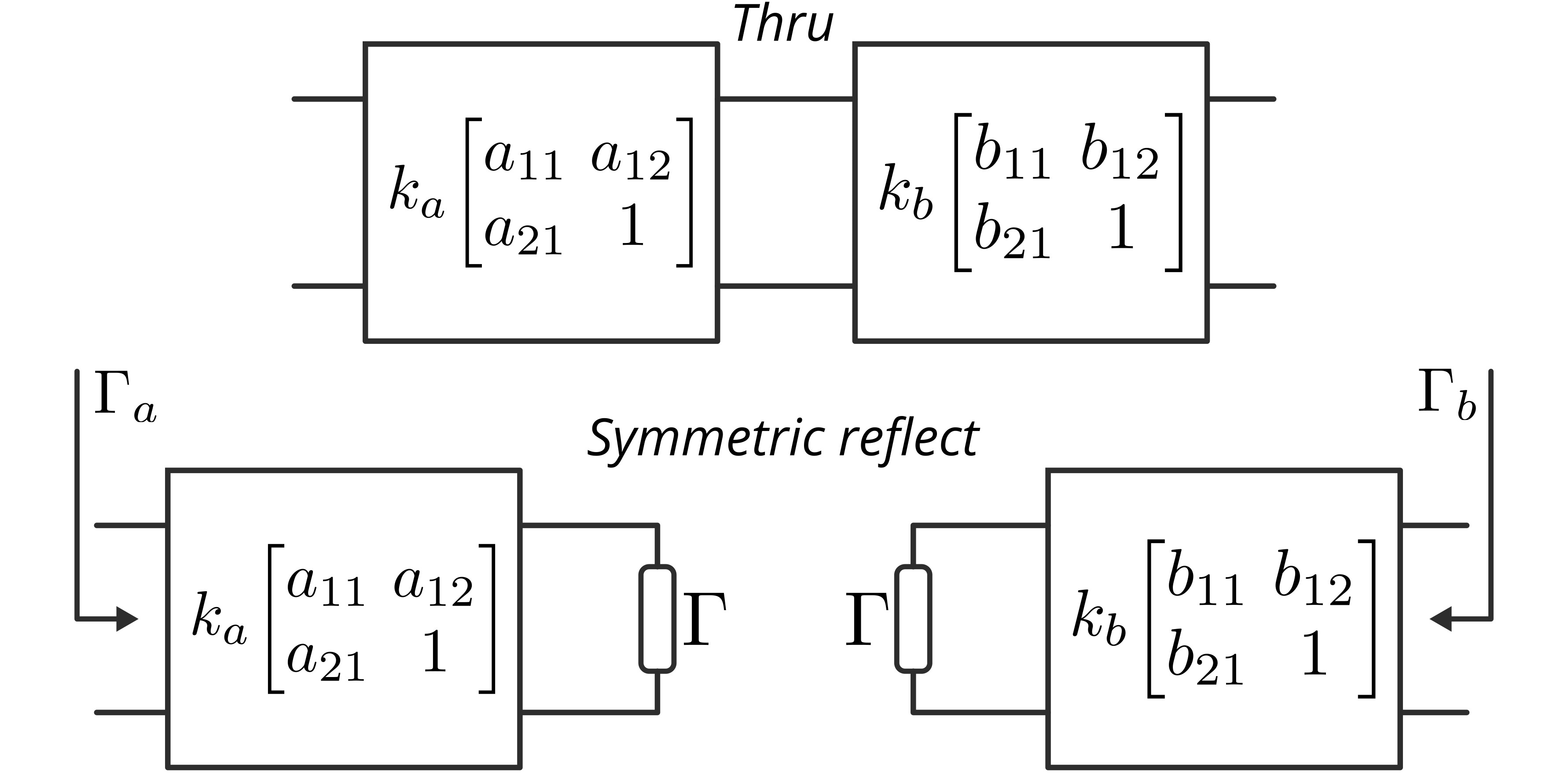Fig. 3. Error box model for the thru and symmetric reflect standard.

Now, with the symmetrical reflect measurement, we can obtain two equations, one for each port, that describe the input reflection coefficient. The equation for the left port is shown below:

\[\Gamma_a = \frac{a_{12}+a_{11}\Gamma}{1+a_{21}\Gamma}\quad\Longrightarrow\quad a_{11}\Gamma=\frac{\Gamma_a-a_{12}}{1-(a_{21}/a_{11})\Gamma_a}, \label{eq:59}\]

and for the right port we have

\[\Gamma_b = \frac{b_{11}\Gamma-b_{21}}{1-b_{12}\Gamma}\quad\Longrightarrow\quad b_{11}\Gamma=\frac{\Gamma_b+b_{21}}{1+(b_{12}/b_{11})\Gamma_b}, \label{eq:60}\]

where $\Gamma_a$ and $\Gamma_b$ represent the raw measurements of the input reflection seen from each port, and $\Gamma$ is the reflection coefficient of the symmetric reflect standard, which is unspecified during calibration.

By combining both \eqref{eq:59} and \eqref{eq:60}, we cancel the term $\Gamma$ and solve for $a_{11}/b_{11}$ as below:

\[\frac{a_{11}\Gamma}{b_{11}\Gamma}=\frac{a_{11}}{b_{11}} = \frac{\Gamma_a-a_{12}}{1-(a_{21}/a_{11})\Gamma_a}\frac{1+(b_{12}/b_{11})\Gamma_b}{\Gamma_b+b_{21}}. \label{eq:61}\]

The solution for $a_{11}$ and $b_{11}$ are determined by using the values of $a_{11}b_{11}$ from \eqref{eq:58} and $a_{11}/b_{11}$ from \eqref{eq:61} as follows:

\[a_{11} = \pm\sqrt{\frac{a_{11}}{b_{11}}a_{11}b_{11}}; \quad b_{11} = a_{11}\frac{b_{11}}{a_{11}}, \label{eq:62}\]

The sign ambiguity is resolved by selecting the answer closest to a known estimate of $\Gamma$. For instance, -1 is used for short standards, while +1 is used for open standards. Any offset should be taken into account using the estimated propagation constant. Finally, with knowledge of $a_{11}$ and $b_{11}$, the denormalization of the error boxes is accomplished through \eqref{eq:42}.

References

[1] R. Marks, “A multiline method of network analyzer calibration,” IEEE Transactions on Microwave Theory and Techniques, vol. 39, no. 7, pp. 1205–1215, 1991, doi: 10.1109/22.85388

[2] D. DeGroot, J. Jargon, and R. Marks, “Multiline trl revealed,” in 60th ARFTG Conference Digest, Fall 2002., pp. 131–155, doi: 10.1109/ARFTGF.2002.1218696

[3] Z. Hatab, M. Gadringer, and W. Bösch, “Improving the reliability of the multiline trl calibration algorithm,” in 2022 98th ARFTG Microwave Measurement Conference (ARFTG), 2022, pp. 1–5, doi: 10.1109/ARFTG52954.2022.9844064

[4] Z. Hatab, M. E. Gadringer and W. Bösch, “Propagation of Linear Uncertainties through Multiline Thru-Reflect-Line Calibration,” in IEEE Transactions on Instrumentation and Measurement, vol. 72, pp. 1-9, 2023, doi: 10.1109/TIM.2023.3296123, e-print doi: 10.48550/arXiv.2301.09126.

[5] J. Brewer, “Kronecker products and matrix calculus in system theory,” IEEE Transactions on Circuits and Systems, vol. 25, no. 9, pp. 772–781, sep 1978, doi: 10.1109/TCS.1978.1084534

[6] M. G. Ali, , S. A. Khan, and S. G. Khawaja, “Finding the unique permutation matrix for reverse order kronecker product intuitively,” International Journal of Computer Theory and Engineering, vol. 11, no. 6, pp. 107–111, 2019, doi: 10.7763/ijcte.2019.v11.1252

[7] C. R. Johnson, “Positive definite matrices,” The American Mathematical Monthly, vol. 77, no. 3, pp. 259–264, mar 1970, doi: 10.2307/2317709

[8] J. Wilkinson, The Algebraic Eigenvalue Problem, ser. Monographs on numerical analysis. Clarendon Press, 1988, ISBN: 9780198534181

[9] C. Eckart and G. Young, “The approximation of one matrix by another of lower rank,” Psychometrika, vol. 1, no. 3, pp. 211–218, sep 1936, doi: 10.1007/BF02288367

[10] A. M. Chebotarev and A. E. Teretenkov, “Singular value decomposition for the takagi factorization of symmetric matrices,” Applied Mathematics and Computation, vol. 234, pp. 380–384, may 2014, doi: 10.1016/j.amc.2014.01.170