Digital MIMO: From SISO to Beamforming
Ok, no one can disagree that beamforming is not cool. But you know what’s cooler? Knowing how it works. This post is based on a lab manual I wrote years ago for a university course on MIMO (Multiple-Input Multiple-Output) systems, in which students implemented the concepts on software-defined radios. While digging through my old files, I came across the manual again and figured the material deserves a second life as a blog post.
The motivation behind MIMO is simple: wireless channels fade, and fading severely degrades the reliability of a single-antenna link. With multiple antennas, the receiver can obtain several independent copies of the same symbol, which is known as diversity. I want to build up this idea step by step, starting from a single-antenna link as the baseline, then adding antennas at the receiver, then at the transmitter, and finally at both ends, ending with beamforming, where the transmitter knows the channel and adapts to it. All the processing happens on the sampled baseband symbols in Digital Signal Processing (DSP), hence the “digital” in the title. Throughout the post I derive the equations behind each configuration, and at the end you will find a Python script that implements them and reproduces the simulation results.
The Wireless Channel
Losses and Fading
The losses a wireless link experiences come in two flavors: path loss and fading [1]. Path loss is just the inverse-square law: the energy of the electromagnetic wave spreads over distance. Fading splits further into large-scale fading, i.e., shadowing from obstacles like buildings, and small-scale fading, which refers to the rapid fluctuations of the received signal caused by interference among the multipath components. The image below illustrates all three effects. Small-scale fading is the one that concerns us in this post: moving the antenna by a fraction of a wavelength can drop the signal by tens of dB.
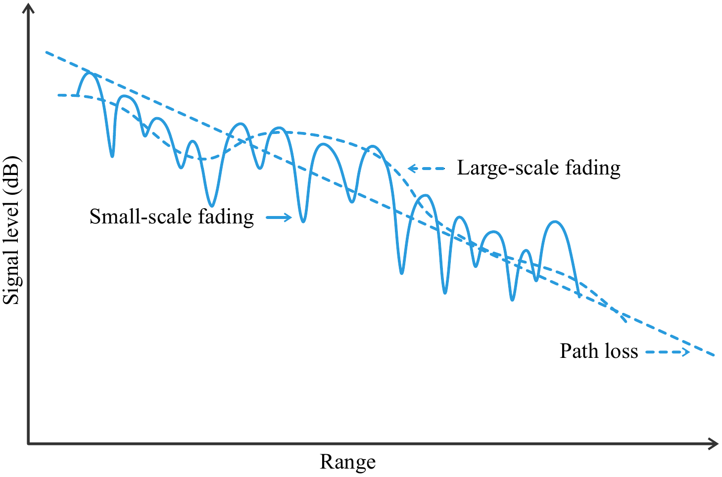 Fig. 1.: Sources of signal degradation in a wireless system (recreation from [1]).
The Narrowband Assumption
The general channel model is a time-variant filter, i.e., the received signal is the convolution of the transmitted signal with the channel impulse response. In discrete time, and with additive noise, the received samples read:
\[y[k] = \sum_{m=0}^{m_\mathrm{total}-1} h[m]\, s[k-m] + n[k] \label{eq:1}\]where $s[k]$ are the transmitted symbols, $h[m]$ is the channel impulse response, and $n[k]$ is zero-mean complex Gaussian noise with variance $N_0/2$ per component. A symbol is a complex number carrying a fixed group of data bits, drawn from a finite set of points called a constellation (e.g., QPSK). Multiple taps in $h[m]$ mean that consecutive symbols smear into each other, known as inter-symbol interference. Luckily, if the signal bandwidth is much smaller than the coherence bandwidth of the channel, the channel is frequency-flat over the band of interest (see Fig. 2), and the entire impulse response collapses into a single complex number. Equation \eqref{eq:1} then simplifies to:
\[y[k] = h\,s[k] + n[k] \label{eq:2}\]where $h$ is called the channel coefficient. This is the narrowband assumption, and it is the foundation of everything that follows. The channel is, of course, also time-variant, but we assume it changes much slower than the processing time, so I drop the time dependence of $h$ for notational simplicity.
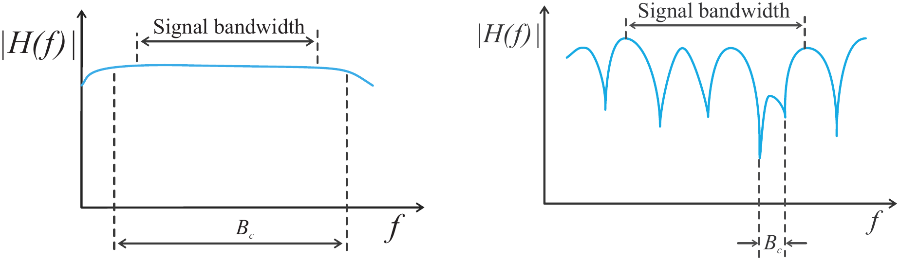 Fig. 2.: Frequency-flat (left) versus frequency-selective (right) channels, where $B_c$ denotes the coherence bandwidth.
A schematic of this single-antenna model, better known as SISO (Single-Input Single-Output), is shown below. One practical remark: in a real single-carrier system, $s[k]$ also contains the pulse shaping filter, and the receiver first applies a matched filter and downsamples to the symbol rate. I assume all of that, including synchronization, has already happened, so Equation \eqref{eq:2} directly describes the received symbols.
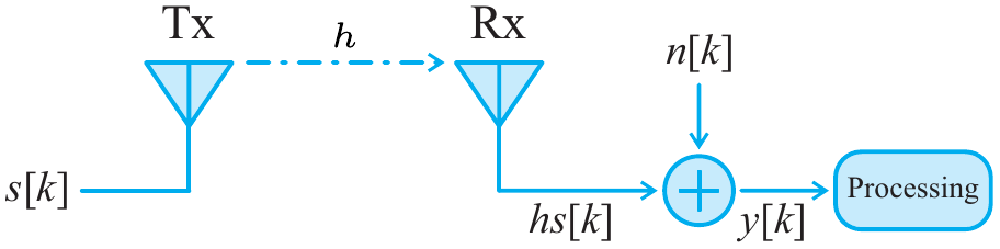 Fig. 3.: The SISO configuration.
If you are wondering how systems with wideband signals deal with frequency-selective channels: the most popular answer is OFDM (Orthogonal Frequency-Division Multiplexing), which splits the band into many narrow subcarriers such that each subcarrier sees a frequency-flat channel. So everything discussed in this post applies to WiFi and cellular systems as well, just per subcarrier.
The SISO Baseline
Symbol Error Ratio
To quantify the impact of fading, we need a performance metric: the Symbol Error Ratio (SER), which is the probability of detecting a wrong symbol. As a reference, we start with the pure AWGN (Additive White Gaussian Noise) channel, i.e., $y = s + n$ without fading. A handy tool for this is the nearest neighbor approximation [3], which states that the error probability of a symbol is dominated by its closest neighbors in the constellation:
\[P_e \approx N_\mathrm{min}\,\mathrm{Q}\!\left(\frac{d_\mathrm{min}}{\sqrt{2N_0}}\right) \label{eq:3}\]where $N_\mathrm{min}$ is the number of neighboring symbols at the minimum distance $d_\mathrm{min}$, and $\mathrm{Q}(x)$ is the Q-function, i.e., the right-tail probability of the standard normal distribution:
\[\mathrm{Q}(x) = \frac{1}{\sqrt{2\pi}}\int_{x}^{\infty} e^{-z^2/2}\,dz \label{eq:4}\]The concrete constellation I use throughout this post is QPSK (Quadrature Phase-Shift Keying), shown in Fig. 4, where each symbol is one of four points in the complex plane and carries 2 bits. Each QPSK symbol has $N_\mathrm{min}=2$ neighbors at distance $d_\mathrm{min}=\sqrt{2E_s}$, where $E_s$ is the symbol energy. Plugging into Equation \eqref{eq:3} gives the well-known result:
\[\mathrm{SER}_\mathrm{AWGN} \approx 2\,\mathrm{Q}\!\left(\sqrt{\mathrm{SNR}}\right), \qquad \mathrm{SNR} = \frac{E_s}{N_0} \label{eq:5}\]where the ratio $\mathrm{SNR} = E_s/N_0$ is the Signal-to-Noise Ratio (SNR). It is the single most important quantity for link performance, and essentially everything that follows is about improving it.
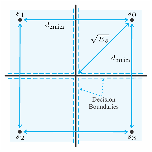 Fig. 4.: QPSK constellation.
Now back to the fading channel of Equation \eqref{eq:2}. Assuming the receiver knows $h$ perfectly, the SNR becomes a function of the channel:
\[\mathrm{SNR}_h = |h|^2\frac{E_s}{N_0} \label{eq:6}\]Since $h$ fluctuates, so does the SNR, and so does the SER. The common assumption is that $\lvert h\rvert$ is Rayleigh distributed with $\EV{\lvert h\rvert^2} = 1$ (Rician distribution would be more general, but the math gets messy!). Then $\mathrm{SNR}_h$ is exponentially distributed, and averaging Equation \eqref{eq:5} over its density delivers the average SER [1]:
\[\overbar{\mathrm{SER}} = \EV{2\,\mathrm{Q}\!\left(\sqrt{\mathrm{SNR}_h}\right)} = 1 - \sqrt{\frac{\overbar{\mathrm{SNR}}}{2+\overbar{\mathrm{SNR}}}}, \qquad \overbar{\mathrm{SNR}} = \frac{E_s}{N_0} \label{eq:7}\]The plot below compares Equations \eqref{eq:5} and \eqref{eq:7}, and the difference is huge. In AWGN, the SER decays rapidly, while in Rayleigh fading it decays with a slope of only one decade per 10 dB, i.e., $\overbar{\mathrm{SER}}\propto 1/\overbar{\mathrm{SNR}}$. At a target SER of $10^{-4}$, the fading channel requires about 28 dB more transmit power. The reason: no matter how much power you transmit, every now and then the channel is in a deep fade and the symbols are lost. The average error rate is dominated by these rare deep fades. This is precisely the problem MIMO diversity solves.
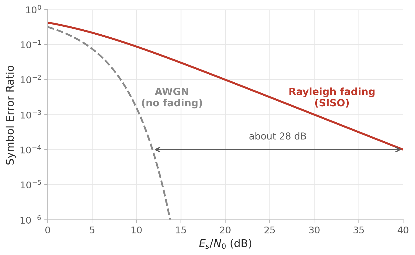 Fig. 5.: SER of QPSK in an AWGN channel versus a Rayleigh fading channel.
Channel Estimation
Until now, I simply assumed that the receiver knows $h$. In practice, the receiver must correct for the rotation and scaling that $h$ introduces (this is called equalization), otherwise the received constellation is rotated arbitrarily and detection fails completely:
\[\hat{s} = \frac{y}{h} = s + \frac{n}{h} \label{eq:8}\]To obtain $h$, we transmit a pilot sequence $\bs{s}_p$ that the receiver knows, collect the corresponding received samples $\bs{y}_p$, and solve for $h$ in the least squares sense:
\[\hat{h} = (\bs{s}_p^H\bs{s}_p)^{-1}\bs{s}_p^H\bs{y}_p = \frac{\bs{s}_p^H\bs{y}_p}{\|\bs{s}_p\|^2} \label{eq:9}\]There are also adaptive methods (Recursive Least Squares, Least Mean Squares, and their variants) that avoid buffering the whole pilot sequence, but plain least squares is all we need here. The figure below summarizes the complete SISO receive chain.
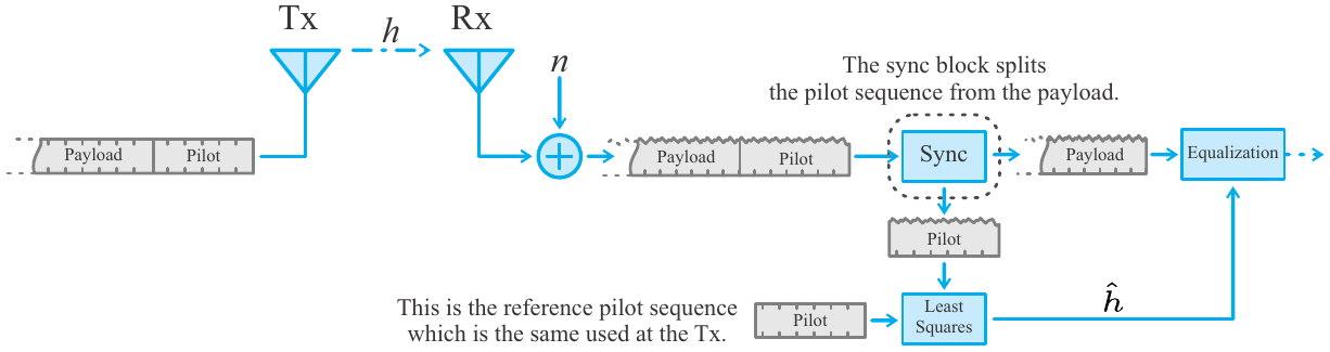 Fig. 6.: Channel estimation and equalization in a wireless SISO system.
SIMO — Receive Diversity
The first upgrade is to add antennas at the receiver, giving a SIMO (Single-Input Multiple-Output) configuration. With $M_R$ receive antennas, each antenna sees its own channel coefficient and its own noise:
\[\underbrace{\begin{bmatrix} y_0\\y_1\\\vdots\\y_{M_R-1} \end{bmatrix}}_{\bs{y}} = \underbrace{\begin{bmatrix} h_0\\h_1\\\vdots\\h_{M_R-1} \end{bmatrix}}_{\bs{h}}s + \underbrace{\begin{bmatrix} n_0\\n_1\\\vdots\\n_{M_R-1} \end{bmatrix}}_{\bs{n}} \label{eq:10}\]One thing that can be confusing is the notion of “SIMO” when talking about multiple receive antennas. When we say single input, we mean the transmitted data is a single stream. Multiple output refers to the number of copies obtained from different paths using the multiple receiver antennas. In other words, input/output counts are read from left (transmitter) to right (receiver), as illustrated in the figure below with sketched transmit and receive antennas.
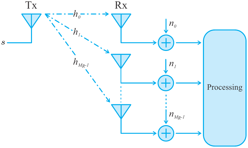 Fig. 7.: Schematic of the SIMO configuration.
The question now is, after obtaining these multiple copies from the different receive antennas, how do we best combine them into a single symbol estimate? Since the model is linear and the noise is Gaussian, least squares is again the answer, and its solution is known in the wireless world as Maximum Ratio Combining (MRC):
\[\hat{s} = (\bs{h}^H\bs{h})^{-1}\bs{h}^H\bs{y} = \frac{\bs{h}^H}{\|\bs{h}\|^2}\bs{y} \label{eq:11}\]The name describes exactly what happens: each copy is weighted by its own channel gain (strong copies count more) and corrected for its phase before summing. Substituting the model \eqref{eq:10} into \eqref{eq:11} shows what MRC does to the noise:
\[\hat{s} = s + \frac{\bs{h}^H}{\|\bs{h}\|^2}\bs{n} \label{eq:12}\]and computing the ratio of signal power to noise power delivers the post-combining SNR:
\[\mathrm{SNR}_\bs{h} = \|\bs{h}\|^2\frac{E_s}{N_0} = \sum_{i=0}^{M_R-1}|h_i|^2\frac{E_s}{N_0} \label{eq:13}\]This is the key result: the SNR is now a sum of $M_R$ independent channel gains. For a deep fade to hurt us, all $M_R$ channels must fade simultaneously, which is far less likely than a single channel fading. Statistically, the sum in Equation \eqref{eq:13} follows an Erlang distribution (sum of independent exponentials), and averaging the QPSK SER over it gives a compact high-SNR approximation [1]. It is worth writing this result in general form, since the same structure appears for every scheme in this post. For a diversity order $L$, when the post-combining SNR is the sum of $L$ independent Rayleigh gains each averaging $\overbar{\mathrm{SNR}} = E_s/N_0$, the average SER is [1]:
\[\overbar{\mathrm{SER}} \approx 2\binom{2L-1}{L}\left(\frac{1}{2\,\overbar{\mathrm{SNR}}}\right)^{L}, \qquad \overbar{\mathrm{SNR}} = \frac{E_s}{N_0} \label{eq:14}\]The exponent $L$ is called the diversity order, and it is the first of two figures of merit that we will track for every configuration in this post, so let me define it properly. The diversity order is the negative slope of the SER curve on a log-log scale [2]:
\[\text{diversity order} = -\frac{\mathrm{d}}{\mathrm{d}\,(\log\overbar{\mathrm{SNR}})}\,(\log\overbar{\mathrm{SER}}) \label{eq:div}\]Intuitively, it counts how many independent copies of the symbol the receiver has to work with. For an error to occur, all $L$ channels must be in a deep fade at the same time, and the probability of that scales as $1/\overbar{\mathrm{SNR}}^L$. So the SER drops $L$ decades for every 10 dB of extra SNR. SISO has diversity order 1, which is the shallow one-decade-per-10-dB slope we saw in Fig. 5, whereas MRC with $M_R$ antennas has diversity order $L = M_R$.
The second figure of merit is the array gain. While diversity bends the slope of the curve, the array gain simply shifts it to the left, i.e., it is the average boost in SNR from coherently combining the copies. It is defined as the ratio of the average post-combining SNR to the single-antenna reference $E_s/N_0$ [2]:
\[\text{array gain} = \frac{\EV{\mathrm{SNR}_\mathrm{post}}}{E_s/N_0} \label{eq:arraygain}\]For MRC, the post-combining SNR is given by Equation \eqref{eq:13}, and using $\EV{\lvert h_i\rvert^2} = 1$ (unit-variance Rayleigh gains) gives $\EV{\lVert\bs{h}\rVert^2} = M_R$, so the array gain equals $M_R$. Putting the two together, two receive antennas make the link more robust against fades (diversity order 2) and, on top of that, collect twice the signal energy on average (array gain 2).
The leading factor 2 in Equation \eqref{eq:14} is the QPSK nearest-neighbor count from Equation \eqref{eq:5}; you often see this formula quoted without it, which is the BPSK (Binary Phase-Shift Keying) version.
The plot below adds the MRC curves to our running comparison. I include both $1\times 2$ and $1\times 4$ MRC so you can see the diversity order directly as the slope: doubling the receive antennas doubles the steepness, and the gap to the fading SISO curve widens quickly.
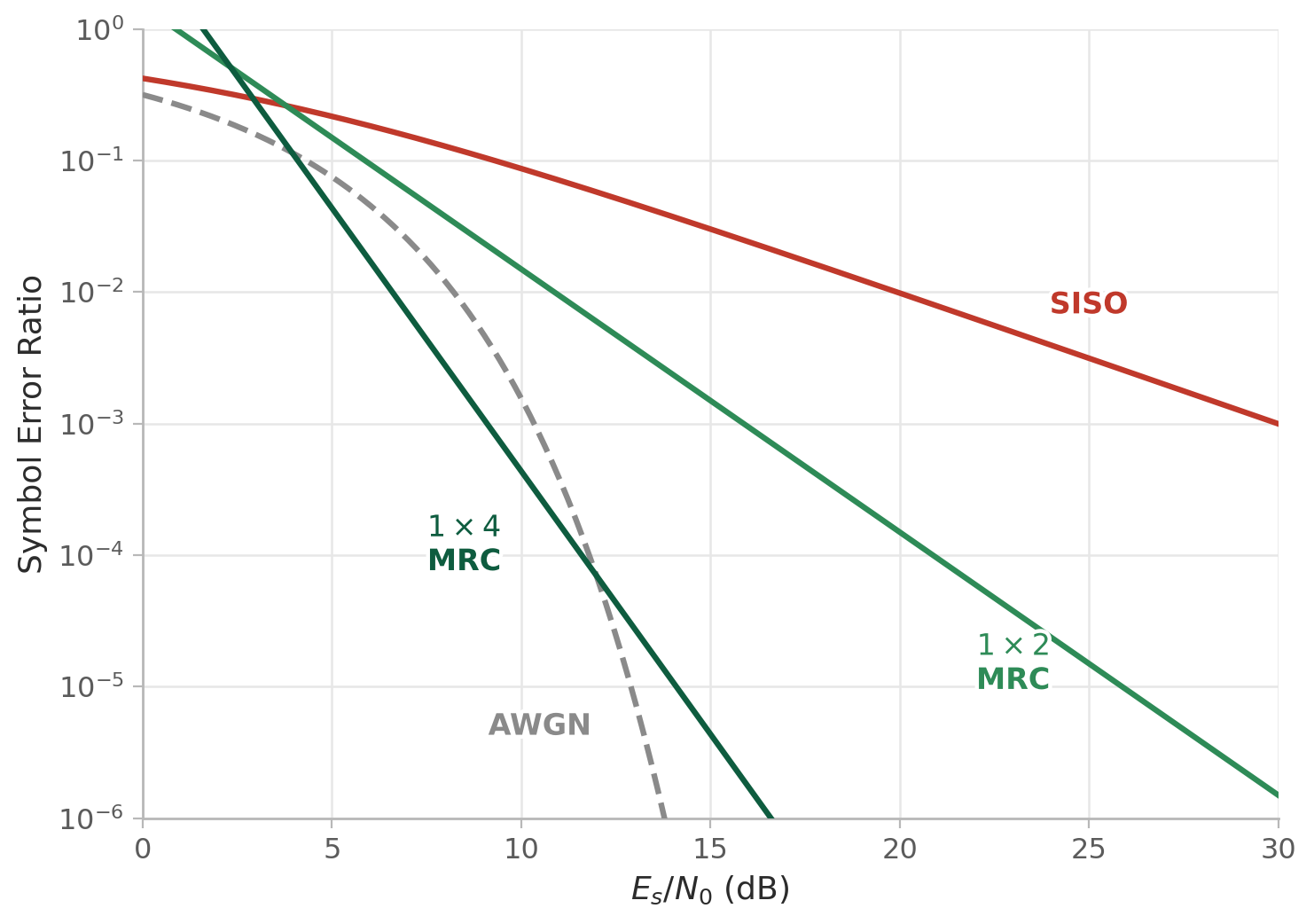 Fig. 8.: SER of QPSK with receive diversity (MRC), compared to the SISO baseline.
MISO — Transmit Diversity
Now we consider the opposite case: multiple antennas at the transmitter and only one at the receiver (MISO, Multiple-Input Single-Output). This case matters in practice because a base station can host many antennas, while a small handheld device often cannot. It is also a fundamentally harder problem from a DSP point of view, because the transmitter does not know the channel, so it cannot pre-weight its antennas the way MRC weights the received copies.
To appreciate the difficulty, consider the naive approach: transmit the same symbol from both antennas (scaled by $1/\sqrt{2}$ to keep the total power fixed), as illustrated below.
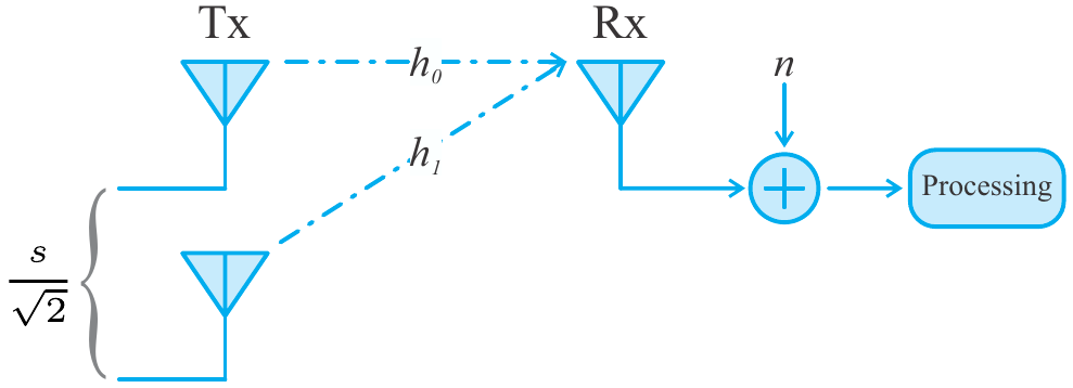 Fig. 9.: The wrong way of doing MISO.
The received signal is then:
\[y = \frac{1}{\sqrt{2}}s\,(h_0+h_1) + n \label{eq:15}\]We are back to the SISO model, just with the combined channel $(h_0+h_1)/\sqrt{2}$. The problem is that the sum of two complex Gaussians is still complex Gaussian, so the combined channel is Rayleigh distributed exactly like before. We gain no diversity at all, despite using two transmitters.
Alamouti’s Scheme
The solution is one of my favorite results in wireless communication, published by Alamouti in 1998 [4], and it belongs to the family of space-time block codes. The idea is to code two symbols across two antennas (space) and two time slots (time), so the data rate is not affected. In the first time slot, the antennas transmit $s_0$ and $s_1$; in the second, they transmit $-s_1^*$ and $s_0^*$ (everything scaled by $1/\sqrt{2}$ for constant total power):
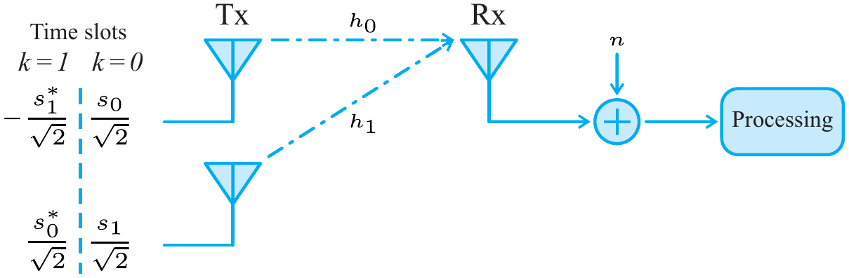 Fig. 10.: Alamouti’s transmission scheme.
Assuming the channel stays constant over the two time slots, the two received samples are:
\[y[0] = \frac{1}{\sqrt{2}}\left(h_0 s_0 + h_1 s_1\right) + n[0], \qquad y[1] = \frac{1}{\sqrt{2}}\left(-h_0 s_1^* + h_1 s_0^*\right) + n[1] \label{eq:16}\]The trick is in the decoding: take the complex conjugate of $y[1]$ and stack it with $y[0]$, and the result is a $2\times 2$ linear system in the original symbols:
\[\underbrace{\begin{bmatrix} y[0]\\y^*[1] \end{bmatrix}}_{\bs{y}} = \underbrace{\frac{1}{\sqrt{2}}\begin{bmatrix} h_0 & h_1\\ h_1^* & -h_0^* \end{bmatrix}}_{\bs{H}_\mathrm{eff}}\underbrace{\begin{bmatrix} s_0\\s_1 \end{bmatrix}}_{\bs{s}} + \underbrace{\begin{bmatrix} n[0]\\n^*[1] \end{bmatrix}}_{\bs{n}} \label{eq:17}\]The effective channel matrix $\bs{H}_\mathrm{eff}$ is special: its columns are orthogonal by construction [2], i.e.:
\[\bs{H}_\mathrm{eff}^H\bs{H}_\mathrm{eff} = \frac{\|\bs{h}\|^2}{2}\,\bs{I}_{2\times2}, \qquad \|\bs{h}\|^2 = |h_0|^2 + |h_1|^2 \label{eq:18}\]which means the least squares solution decouples the two symbols perfectly, without any noise enhancement:
\[\hat{\bs{s}} = (\bs{H}_\mathrm{eff}^H\bs{H}_\mathrm{eff})^{-1}\bs{H}_\mathrm{eff}^H\bs{y} = \frac{2}{\|\bs{h}\|^2}\bs{H}_\mathrm{eff}^H\bs{y} \label{eq:19}\]Following the same steps as in the MRC case, the post-decoding SNR comes out as:
\[\mathrm{SNR}_\bs{h} = \frac{\|\bs{h}\|^2}{2}\frac{E_s}{N_0} \label{eq:20}\]Compare this with Equation \eqref{eq:13}: it is the $1\times 2$ MRC result with the SNR scaled down by 2. So Alamouti achieves the same diversity order ($L = 2$, the same slope) as $1\times 2$ MRC, but the halved SNR shifts its curve 3 dB to the right, which you get by substituting $\overbar{\mathrm{SNR}} \to \overbar{\mathrm{SNR}}/2$ in Equation \eqref{eq:14}. Its array gain is therefore 1, i.e., no array gain. The 3 dB penalty comes from the transmitter not knowing the channel: the power is split equally between the two antennas, regardless of which channel is better. Still, it is fascinating that a simple manipulation of the transmitted symbols achieves diversity without affecting the data rate.
The plot below makes the comparison concrete. The $2\times1$ Alamouti curve runs parallel to $1\times2$ MRC, since both have diversity order 2 and therefore the same slope, but it is shifted 3 dB to the right because it lacks the array gain. Either way, both are a large improvement over the fading SISO baseline.
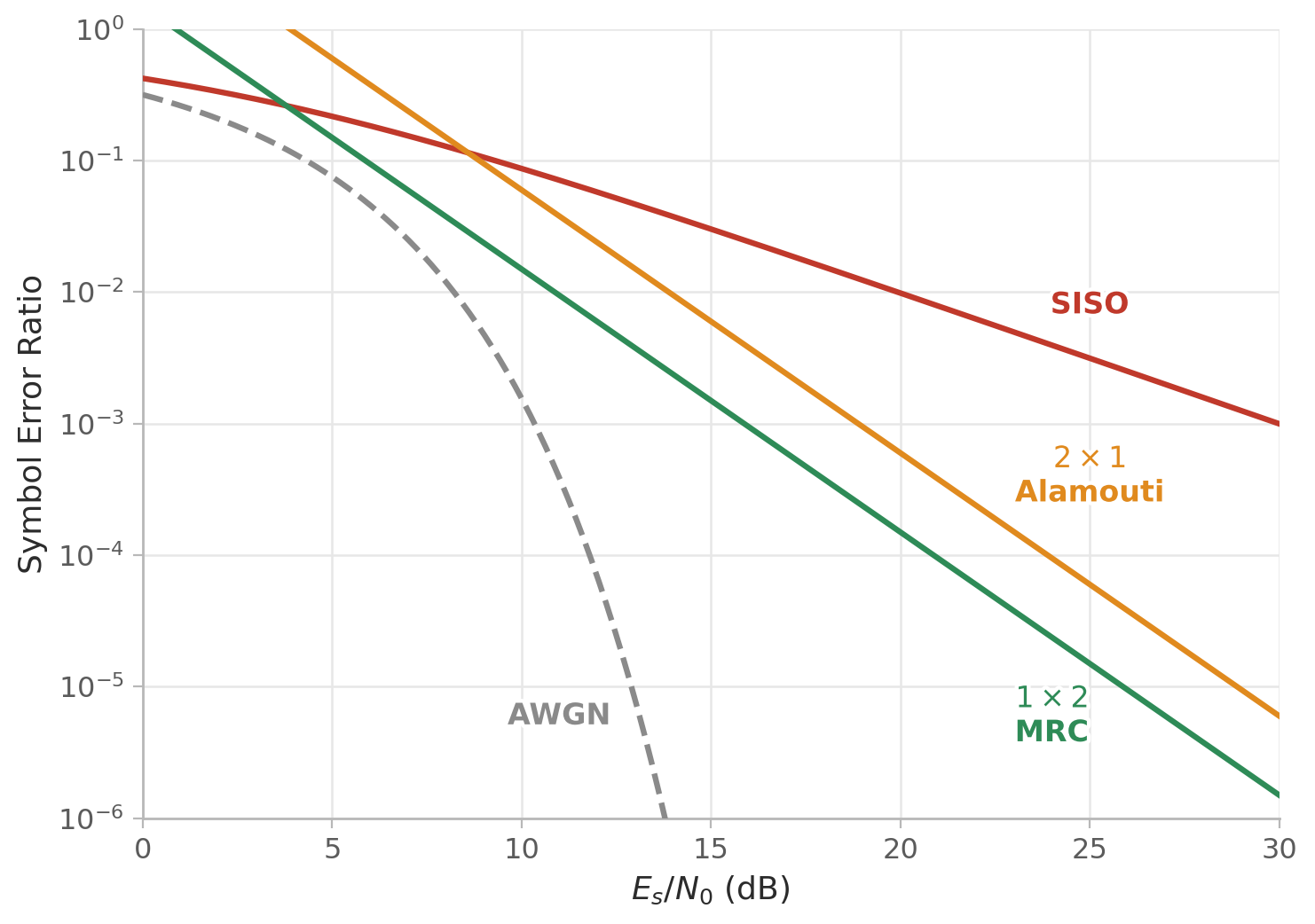 Fig. 11.: SER of QPSK with transmit diversity ($2\times1$ Alamouti), compared to $1\times2$ MRC and the SISO baseline.
There is also a practical subtlety in channel estimation. The receiver needs $h_0$ and $h_1$ separately to build $\bs{H}_\mathrm{eff}$, but if both transmitters send their pilots simultaneously, they interfere exactly as in Equation \eqref{eq:15}. The solution is orthogonal pilot sequences, i.e., $\bs{s}_{p0}^H\bs{s}_{p1} = 0$. The simplest construction: take the SISO pilot and zero-pad it, as a suffix for one antenna and as a prefix for the other.
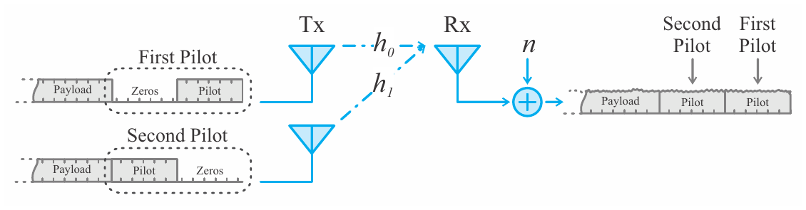 Fig. 12.: Orthogonal pilots for channel estimation in the 2×1 MISO configuration.
MIMO — Combining Alamouti with MRC
If transmit diversity and receive diversity each work on their own, nothing stops us from using both. With $M_T = 2$ transmitters running Alamouti’s scheme and $M_R$ receivers each performing the stacking trick of Equation \eqref{eq:17}, every receiver $i$ contributes its own effective channel matrix, and we simply stack them all:
\[\underbrace{\begin{bmatrix} \bs{y}_0\\\vdots\\\bs{y}_{M_R-1} \end{bmatrix}}_{\bs{y}} = \underbrace{\begin{bmatrix} \bs{H}_{\mathrm{eff}_0}\\\vdots\\\bs{H}_{\mathrm{eff}_{M_R-1}} \end{bmatrix}}_{\bs{H}_\mathrm{eff}}\bs{s} + \underbrace{\begin{bmatrix} \bs{n}_0\\\vdots\\\bs{n}_{M_R-1} \end{bmatrix}}_{\bs{n}} \label{eq:21}\]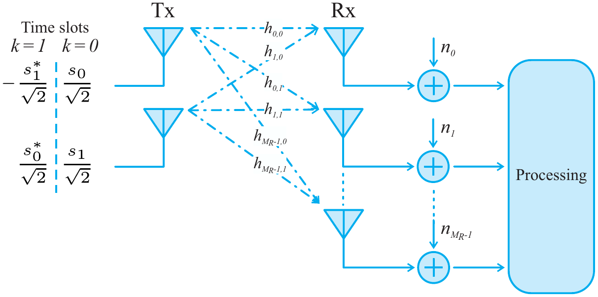 Fig. 13.: Combining Alamouti’s scheme at the transmitter with MRC at the receiver.
The stacked matrix inherits the orthogonality, with the gains of all receivers accumulating, so the least squares decoder has the same one-liner structure as Equation \eqref{eq:19}, and the post-decoding SNR becomes:
\[\mathrm{SNR}_\bs{h} = \frac{1}{2}\sum_{i=0}^{M_R-1}\left(|h_{i0}|^2 + |h_{i1}|^2\right)\frac{E_s}{N_0} \label{eq:22}\]That is a sum over $2M_R$ independent channel gains, each at half power: diversity order $L = 2M_R$ and array gain $M_R$. The diversity order has a clean interpretation here: each of the two transmit antennas has its own path to each of the $M_R$ receive antennas, so there are $2M_R$ independent paths in total, and the diversity order counts exactly these paths. For the common symmetric $2\times2$ case (found in many WiFi devices), that means diversity order 4.
The plot below adds the $2\times2$ Alamouti curve. Its slope is now twice as steep as the diversity-2 curves ($1\times2$ MRC and $2\times1$ Alamouti), which is the signature of doubling the diversity order.
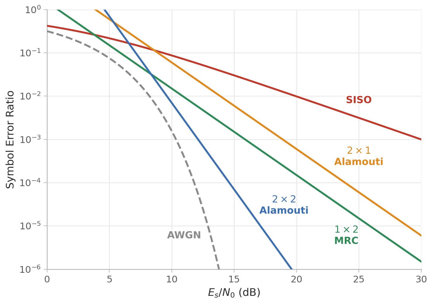 Fig. 14.: SER of QPSK for the $2\times2$ Alamouti MIMO configuration, compared to the previous schemes.
Beamforming — When the Transmitter Knows the Channel
Everything so far assumed the transmitter has no knowledge of the channel. Now assume the receiver feeds the channel state information back to the transmitter (or the transmitter infers it from reciprocity). With this knowledge, the transmitter can pre-scale the symbol at each antenna with a complex weight $w_i$, chosen such that the transmissions add up constructively at the receiver. This is beamforming, and since the weights are applied to the baseband samples in DSP, it is digital beamforming (as opposed to the analog phase shifters of a classic phased array).
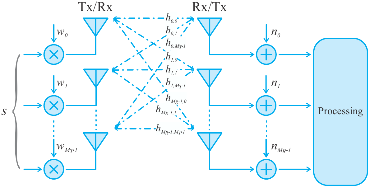 Fig. 15.: MIMO beamforming with M_T transmitters and M_R receivers.
With $M_T$ transmit weights collected in the vector $\bs{w}$ and the channel coefficients arranged in the $M_R\times M_T$ channel matrix $\bs{H}$, the received signal reads:
\[\bs{y} = \bs{H}\bs{w}\,s + \bs{n} \label{eq:23}\]For a fixed $\bs{w}$, the product $\bs{H}\bs{w}$ is just an effective SIMO channel, so the receiver applies MRC as in Equation \eqref{eq:11}:
\[\hat{s} = \frac{(\bs{H}\bs{w})^H}{\|\bs{H}\bs{w}\|^2}\bs{y} \qquad\Longrightarrow\qquad \mathrm{SNR}_\bs{H} = \|\bs{H}\bs{w}\|^2\frac{E_s}{N_0} \label{eq:24}\]The interesting question is how to pick $\bs{w}$. Naturally, we want to maximize the SNR, under the constraint that beamforming does not increase the transmit power:
\[\bs{w}_\mathrm{opt} = \arg\max_{\bs{w}}\ \|\bs{H}\bs{w}\|^2, \qquad \text{subject to}\ \|\bs{w}\|^2 = 1 \label{eq:25}\]This optimization problem can be solved with the Lagrange multiplier method. Setting the derivative of $\lVert\bs{H}\bs{w}\rVert^2 - \lambda(\lVert\bs{w}\rVert^2-1)$ with respect to $\bs{w}$ to zero yields:
\[\bs{H}^H\bs{H}\,\bs{w}_\mathrm{opt} = \lambda\,\bs{w}_\mathrm{opt} \label{eq:26}\]which you should recognize as an eigenvalue problem: the candidates for $\bs{w}_\mathrm{opt}$ are the eigenvectors of $\bs{H}^H\bs{H}$. Multiplying Equation \eqref{eq:26} from the left with $\bs{w}_\mathrm{opt}^H$ and using $\lVert\bs{w}_\mathrm{opt}\rVert^2=1$ reveals which one to take:
\[\|\bs{H}\bs{w}_\mathrm{opt}\|^2 = \lambda \qquad\Longrightarrow\qquad \mathrm{SNR}_\bs{H} = \lambda_\mathrm{max}\frac{E_s}{N_0} \label{eq:27}\]So the optimal beamformer is the eigenvector of $\bs{H}^H\bs{H}$ corresponding to its largest eigenvalue $\lambda_\mathrm{max}$ (all eigenvalues are real and non-negative, since $\bs{H}^H\bs{H}$ is Hermitian and positive semi-definite). In practice, you compute it via the singular value decomposition $\bs{H} = \bs{U}\bs{\Sigma}\bs{V}^H$: the right singular vector belonging to the largest singular value is exactly $\bs{w}_\mathrm{opt}$, and $\lambda_\mathrm{max} = \sigma_\mathrm{max}^2$. Note that eigenvectors are only defined up to a unit complex scalar, so different implementations may return versions differing by a phase — the beamforming direction, which is what we care about, stays the same.
A special case worth highlighting is $M_R = 1$, i.e., MISO with channel knowledge at the transmitter. The channel matrix collapses to a row vector $\bs{h}^H$, and maximizing $\lvert\bs{h}^H\bs{w}\rvert^2$ has an obvious geometric answer: point $\bs{w}$ in the same direction as $\bs{h}$.
\[\bs{w}_\mathrm{opt} = \frac{\bs{h}}{\|\bs{h}\|} \qquad\Longrightarrow\qquad \mathrm{SNR}_\bs{h} = \|\bs{h}\|^2\frac{E_s}{N_0} \label{eq:28}\]This configuration is called Maximum Ratio Transmission (MRT), and its performance is identical to MRC — compare with Equation \eqref{eq:13}. In other words, with channel knowledge, the transmitter fully recovers the 3 dB that Alamouti’s scheme loses. This configuration is common at cellular base stations, where many antennas can be installed, while the handheld device only needs a single antenna.
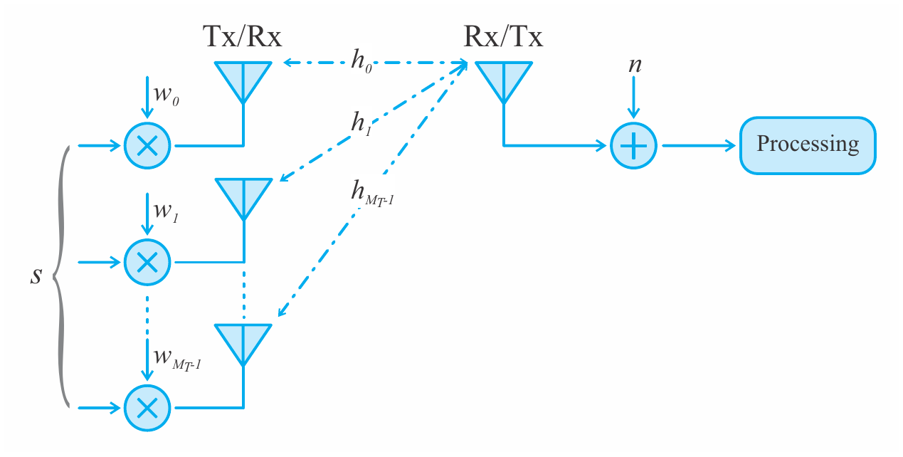 Fig. 16.: MISO beamforming, also known as Maximum Ratio Transmission (MRT).
For the general $M_T\times M_R$ case, the SER has no simple closed form, but $\lambda_\mathrm{max}$ can be bounded from both sides [2]:
\[\frac{\|\bs{H}\|_F^2}{\min(M_T, M_R)} \leqslant \lambda_\mathrm{max} \leqslant \|\bs{H}\|_F^2 \label{eq:29}\]where $\lVert\bs{H}\rVert_F^2$ is the squared Frobenius norm, i.e., the sum of all $M_TM_R$ channel gains. Both bounds are sums of $M_TM_R$ independent Rayleigh gains, so beamforming achieves the full diversity order $M_TM_R$, with an array gain between $M_TM_R/\min(M_T,M_R)$ and $M_TM_R$. Note that for $M_T = 2$, beamforming’s worst case (the lower bound on $\lambda_\mathrm{max}$) gives exactly the $2\times2$ Alamouti curve, so with channel knowledge beamforming is never worse than Alamouti, only better. The table below summarizes all configurations, where CU/CK stands for channel unknown/known to the transmitter.
| Configuration | Diversity order | Array gain |
|---|---|---|
| SISO | $1$ | $1$ |
| SIMO (MRC) | $M_R$ | $M_R$ |
| MISO (CU, Alamouti) | $M_T$ | $1$ |
| MISO (CK, MRT) | $M_T$ | $M_T$ |
| MIMO (CU, Alamouti + MRC) | $M_RM_T$ | $M_R$ |
| MIMO (CK, beamforming) | $M_RM_T$ | $\EV{\lambda_\mathrm{max}}$ |
The plot below puts all the schemes together. Beamforming (the shaded band between its two bounds) achieves the same diversity order as $2\times2$ Alamouti but sits to its left, thanks to the extra array gain from knowing the channel. Notice how close it gets to the AWGN curve, i.e., the no-fading ideal: with enough antennas and channel knowledge, the fading channel can be made to behave almost like an AWGN one.
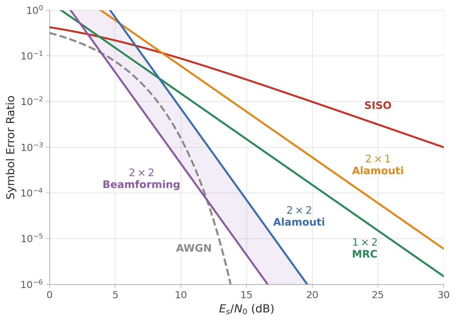 Fig. 17.: SER of QPSK for all discussed configurations. The shaded region marks the theoretical bounds for $2\times2$ beamforming.
Of course, beamforming has its price: the transmitter needs the channel state information, which means either a feedback link from the receiver or channel reciprocity — and the channel must not change faster than you can track it.
Python Simulation
Time to verify all these claims with a Monte Carlo (MC) simulation. The script below implements every scheme discussed in this post using plain NumPy (SciPy is only used for the erfc function): QPSK symbols run through independent Rayleigh channel draws, each receiver structure estimates the symbols exactly with the equations derived above, and the errors are counted. The channel is assumed perfectly known where needed, i.e., no pilots or synchronization are simulated.
1
2
3
4
5
6
7
8
9
10
11
12
13
14
15
16
17
18
19
20
21
22
23
24
25
26
27
28
29
30
31
32
33
34
35
36
37
38
39
40
41
42
43
44
45
46
47
48
49
50
51
52
53
54
55
56
57
58
59
60
61
62
63
64
65
66
67
68
69
70
71
72
73
74
75
76
77
78
79
80
81
82
83
84
85
86
87
88
89
90
91
92
93
import numpy as np
import matplotlib.pyplot as plt
from math import comb
from scipy.special import erfc

rng = np.random.default_rng(42)

def qpsk(N):
    """Random QPSK symbols with unit energy."""
    return ((2*rng.integers(0, 2, N) - 1) + 1j*(2*rng.integers(0, 2, N) - 1))/np.sqrt(2)

def rayleigh(*shape):
    """Complex channel coefficients with Rayleigh magnitude and E{|h|^2} = 1."""
    return (rng.standard_normal(shape) + 1j*rng.standard_normal(shape))/np.sqrt(2)

def awgn(N0, *shape):
    """Zero-mean complex Gaussian noise with variance N0/2 per component."""
    return np.sqrt(N0/2)*(rng.standard_normal(shape) + 1j*rng.standard_normal(shape))

def ser(s, s_hat):
    """Count QPSK symbol errors by comparing the signs of both components."""
    return np.mean((np.sign(s_hat.real) != np.sign(s.real)) | (np.sign(s_hat.imag) != np.sign(s.imag)))

def sim_awgn(N0, N):
    s = qpsk(N)
    return ser(s, s + awgn(N0, N))

def sim_siso(N0, N):
    s = qpsk(N)
    h = rayleigh(N)
    y = h*s + awgn(N0, N)
    return ser(s, y/h)  # zero-forcing equalization

def sim_mrc(N0, N, Mr=2):
    s = qpsk(N)
    h = rayleigh(Mr, N)
    y = h*s + awgn(N0, Mr, N)
    s_hat = np.sum(h.conj()*y, axis=0)/np.sum(np.abs(h)**2, axis=0)
    return ser(s, s_hat)

def sim_alamouti(N0, N, Mr=1):
    s0, s1 = qpsk(N), qpsk(N)                    # two symbols per Alamouti block
    h0, h1 = rayleigh(Mr, N), rayleigh(Mr, N)    # channel constant over two time slots
    y0 = (h0*s0 + h1*s1)/np.sqrt(2) + awgn(N0, Mr, N)                 # time slot k=0
    y1 = (-h0*s1.conj() + h1*s0.conj())/np.sqrt(2) + awgn(N0, Mr, N)  # time slot k=1
    # least squares decoding written out explicitly
    gain = np.sum(np.abs(h0)**2 + np.abs(h1)**2, axis=0)
    s0_hat = np.sqrt(2)*np.sum(h0.conj()*y0 + h1*y1.conj(), axis=0)/gain
    s1_hat = np.sqrt(2)*np.sum(h1.conj()*y0 - h0*y1.conj(), axis=0)/gain
    return (ser(s0, s0_hat) + ser(s1, s1_hat))/2

def sim_beamforming(N0, N, Mt=2, Mr=2):
    s = qpsk(N)
    H = rayleigh(N, Mr, Mt)
    w = np.linalg.svd(H)[2][:, 0, :].conj()   # right singular vector of largest singular value
    g = np.einsum('nij,nj->ni', H, w)         # effective channel H@w
    y = g*s[:, None] + awgn(N0, N, Mr)
    s_hat = np.sum(g.conj()*y, axis=1)/np.sum(np.abs(g)**2, axis=1)
    return ser(s, s_hat)

def qfunc(x):
    return 0.5*erfc(x/np.sqrt(2))

def ser_fading(snr, L, loss=1):
    """High-SNR approximation of the average QPSK SER in Rayleigh fading
    with diversity order L and an SNR penalty factor 'loss'."""
    return 2*comb(2*L - 1, L)*(2*snr/loss)**(-L)

if __name__ == '__main__':
    N = 500_000                        # symbols per Monte Carlo run
    snr_dB = np.linspace(0, 30, 200)   # for the theoretical curves
    snr = 10**(snr_dB/10)
    snr_sim_dB = np.arange(0, 31, 2)   # simulated points

    schemes = [  # (label, simulator, theoretical SER)
        ('AWGN (no fading)',         sim_awgn,     2*qfunc(np.sqrt(snr))),
        ('SISO',                     sim_siso,     1 - np.sqrt(snr/(2 + snr))),
        (r'$1\times 2$ MRC',         sim_mrc,      ser_fading(snr, L=2)),
        (r'$2\times 1$ Alamouti',    sim_alamouti, ser_fading(snr, L=2, loss=2)),
        (r'$2\times 2$ Alamouti',    lambda N0, N: sim_alamouti(N0, N, Mr=2), ser_fading(snr, L=4, loss=2)),
        (r'$2\times 2$ Beamforming', sim_beamforming, ser_fading(snr, L=4)),  # optimistic bound
    ]

    for i, (label, simulate, theory) in enumerate(schemes):
        ser_sim = [simulate(10**(-x/10), N) for x in snr_sim_dB]
        plt.semilogy(snr_dB, theory, color=f'C{i}', label=label)     # theory
        plt.semilogy(snr_sim_dB, ser_sim, 'o', color=f'C{i}', mfc='none')  # simulation
    plt.xlabel(r'$E_s/N_0$ (dB)')
    plt.ylabel('Symbol Error Ratio')
    plt.ylim([1e-6, 1])
    plt.legend()
    plt.grid(True)
    plt.show()
Running the script (it can take a few minutes) produces a plot similar to the one below. The lines are the theoretical curves, and the circles are the simulated values. Note, at low SNR the markers (i.e., MC simulation) sit below the lines, simply because Equation \eqref{eq:14} is a high-SNR approximation (and the nearest-neighbor approximation double-counts corner events in AWGN).
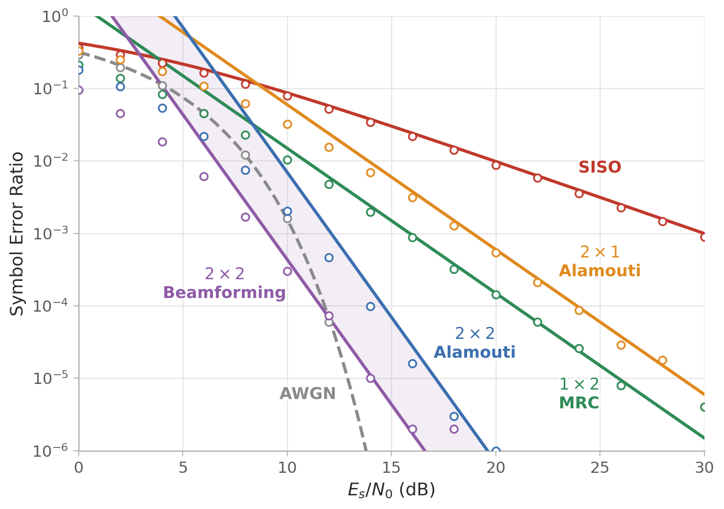 Fig. 18.: SER of all discussed configurations. Lines are theory, circles are simulation, and the shaded region marks the theoretical bounds for 2×2 beamforming.
Be careful when comparing with the literature: the diversity SER approximations are often quoted for BPSK, where the leading nearest-neighbor factor is 1 instead of the 2 in Equation \eqref{eq:14}. It is always a good idea to verify such formulas against a simulation.
Final Remarks
Everything in this post used multiple antennas (i.e., diversity) for one purpose: reliability. The other famous use of MIMO is spatial multiplexing, where the transmit antennas send different symbol streams in parallel to increase the data rate. Diversity and multiplexing are two ends of a fundamental trade-off, and modern systems (WiFi, 5G) switch between them adaptively. Add to that the trend of scaling up to massive MIMO arrays, and it is clear why modern wireless systems keep adding more antennas. But there is more to explore beyond this post. And hopefully you can now appreciate how much DSP goes into adding more antennas, and the tools the industry relies on to keep your wireless link reliable (most of the time 😉).
References
[1] A. F. Molisch, Wireless Communications, 2nd ed. Chichester, UK: Wiley – IEEE, 2010, ISBN: 9780470741863.
[2] A. Paulraj, R. Nabar, and D. Gore, Introduction to Space-Time Wireless Communications. Cambridge, UK: Cambridge University Press, 2003, ISBN: 9780521826150.
[3] J. G. Proakis and M. Salehi, Digital Communications, 5th ed. New York, NY: McGraw-Hill, 2008, ISBN: 9780072957167.
[4] S. M. Alamouti, “A simple transmit diversity technique for wireless communications,” IEEE Journal on Selected Areas in Communications, vol. 16, no. 8, pp. 1451-1458, Oct. 1998, doi: 10.1109/49.730453.