
If you ever find yourself using a simple vector network analyzer (VNA) that can only take $S_{11}$ and $S_{21}$ measurements, this explanation might be an eye-opener on how to calibrate such a system and the assumptions you can make to get accurate results.
This blog was inspired by examples provided by the folks at Scikit-rf [1], and the Math Reference of METAS VNA Tools [2]. In summary, the calibration of a two-port/one-path VNA is essentially a half SOLT (Short-Open-Load-Thru) calibration. However, you still need fully defined Short, Open, Load (SOL) standards and a fully defined two-port standard (often a Thru standard is used).
It’s important to note that most modern VNAs operate in full-reflectometry mode, and some use half-reflectometry with switches to obtain two-port measurements. This tutorial is specific to the case where no switches are used (hence one-path). To make the content more approachable, I will use vector-matrix notations as much as possible. You can find a sample code demonstrating the math presented here on my GitHub: https://github.com/ZiadHatab/two-port-one-path-calibration.
The Block Diagram
As with any VNA calibration topic, we start by examining the block diagram that illustrates the error boxes of the VNA. Please note that, for simplicity, we will disregard any cross-talk terms.
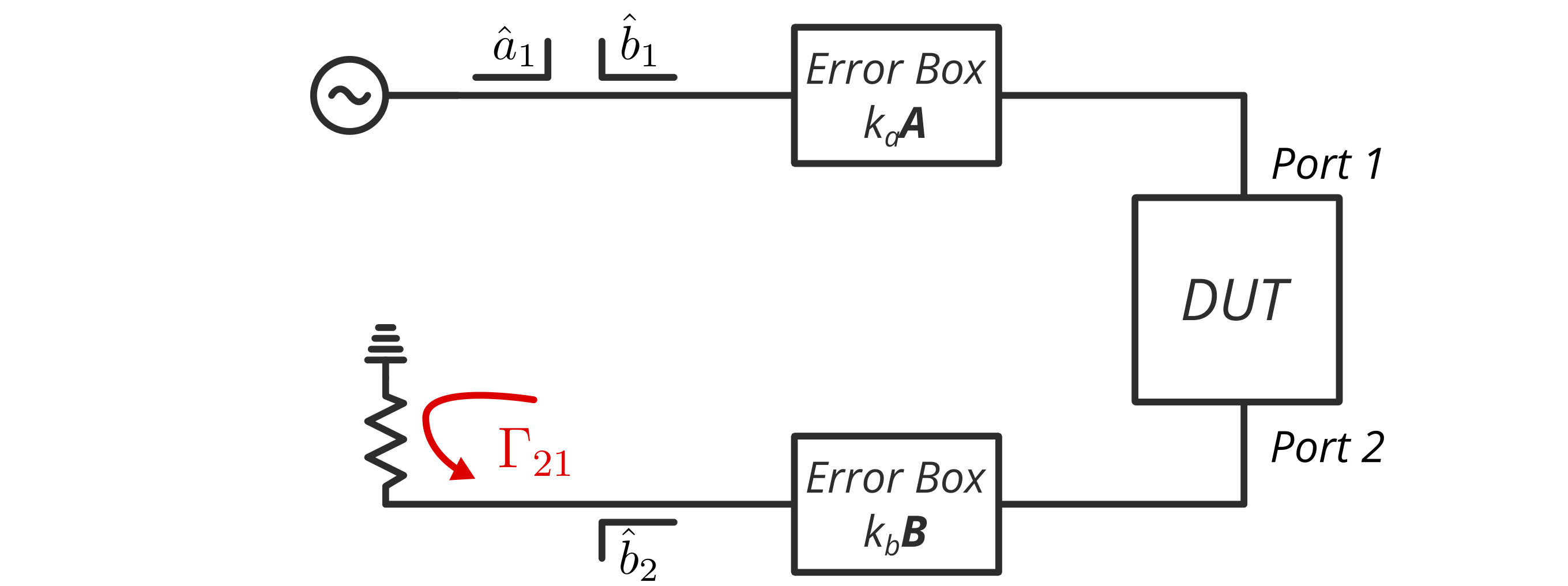 Error box model of a two-port VNA with one-path source excitation.
Because it is a one-path measurement, we only have one set of measurements of the waves $\hat{a}_1, \hat{b}_1, \hat{b}_2$. We can express this relationship using matrix-vector notation with T-parameters as follows:
\[\begin{bmatrix} \hat{b}_1\\ \hat{a}_1 \end{bmatrix} = \underbrace{k_ak_b}_{k}\boldsymbol{A}\boldsymbol{T}_\mathrm{dut}\boldsymbol{B}\begin{bmatrix} \hat{a}_2\\ \hat{b}_2 \end{bmatrix} \label{eq:1}\]where $\hat{a}_2$ represents the incident signal that would have been measured if there was a coupler to measure it at port 2. The error boxes A and B are defined as follows:
\[\boldsymbol{A} = \begin{bmatrix} a_{11} & a_{12}\\ a_{21} & 1 \end{bmatrix}; \qquad \boldsymbol{B} = \begin{bmatrix} b_{11} & b_{12}\\ b_{21} & 1 \end{bmatrix} \label{eq:2}\]The scalars $k_a$ and $k_b$ are factored from the matrices A and B for simplicity, as they can be combined as $k = k_a k_b$. The T matrix in the middle represents the device under test (DUT) or the standards to be measured.
Currently, the measurement in Equation \eqref{eq:1} provides wave parameters. To eliminate the term $\hat{a}_2$ from the equation, S-parameters are used to describe the measurements. By dividing both sides of the equation by $\hat{a}_1$, we can determine the measurement of $S_{11}$ and $S_{21}$, resulting in the following expression:
\[\begin{bmatrix} \hat{b}_1/\hat{a}_1\\ \hat{a}_1/\hat{a}_1 \end{bmatrix} = k\boldsymbol{A}\boldsymbol{T}_\mathrm{dut}\boldsymbol{B}\begin{bmatrix} \hat{a}_2/\hat{a}_1\\ \hat{b}_2/\hat{a}_1 \end{bmatrix}\quad\Longrightarrow\quad \begin{bmatrix} S_{11}\\ 1 \end{bmatrix} = k\boldsymbol{A}\boldsymbol{T}_\mathrm{dut}\boldsymbol{B}\begin{bmatrix} \hat{a}_2/\hat{a}_1\\ S_{21} \end{bmatrix} \label{eq:3}\]We can simplify the ratio $\hat{a}_2/\hat{a}_1$ by expressing it in terms of the termination reflection coefficient $\Gamma_{21}$ as follows:
\[\frac{\hat{a}_2}{\hat{a}_1} = \frac{\hat{a}_2\hat{b}_2}{\hat{a}_1\hat{b}_2} = S_{21}\Gamma_{21}, \qquad \text{where...}\ \Gamma_{21} = \frac{\hat{a}_2}{\hat{b}_2} \label{eq:4}\]Therefore, the measurements can be written as follows:
\[\begin{bmatrix} S_{11}\\ 1 \end{bmatrix} = k\boldsymbol{A}\boldsymbol{T}_\mathrm{dut}\boldsymbol{B}\begin{bmatrix} \Gamma_{21}\\ 1 \end{bmatrix}S_{21} \label{eq:5}\]Note that $\Gamma_{21}$ is constant and can be treated as part of the error terms.
Solving the Error Terms
In total, we can solve for five error terms by using SOL standards and a thru connection (or any known 2-port device). We begin with the SOL standards, which are one-port devices that help us determine the error terms in the matrix A. This matrix consists of three error terms. The block diagram below illustrates the measurement concept.
 Illustration of one-port measurement.
The way we describe the measurement given a connected device is as follows:
\[S_{11}^{(i)} = \frac{a_{11}\Gamma^{(i)} + a_{12}}{a_{21}\Gamma^{(i)} + 1} \label{eq:6}\]where $\Gamma^{(i)}$ describes the actual reflection of the connected device (i.e., known value) and $S_{11}^{(i)}$ is the corresponding measurement. The superscript $(\cdot)^{(i)}$ indicates the $i$-th measured device. This relationship is known as a linear fractional transform, or a Möbius transform. For more information, you can refer to [3]. The term $k_a$ does not appear in the equation because it appears in both the numerator and denominator, canceling out and therefore not mentioned.
For the solution of the error terms $a_{11}, a_{12}, a_{21}$, they can be solved by solving the linear system of equations below:
\[\begin{bmatrix} \Gamma^{(1)} & 1 & -S_{11}^{(1)}\Gamma^{(1)} \\[.5mm] \Gamma^{(2)} & 1 & -S_{11}^{(2)}\Gamma^{(2)} \\[.5mm] \Gamma^{(3)} & 1 & -S_{11}^{(3)}\Gamma^{(3)} \end{bmatrix} \begin{bmatrix} a_{11}\\ a_{12}\\ a_{21} \end{bmatrix} = \begin{bmatrix}S_{11}^{(1)}\\S_{11}^{(2)}\\S_{11}^{(3)}\end{bmatrix} \label{eq:7}\]where superscripts 1, 2, and 3 correspond to open, short, and load standards in no particular order. The solution for $a_{11}, a_{12}, a_{21}$ can be obtained by taking the inverse of the system matrix.
Now that we have solved for the matrix A, we can proceed to solve for two more error terms using the thru standard (or any known two-port device). Recall the equation that describes the measurement of a two-port device under the one-path model:
\[\begin{bmatrix} S_{11}\\ 1 \end{bmatrix} = k\boldsymbol{A}\boldsymbol{T}_\mathrm{thru}\boldsymbol{B}\begin{bmatrix} \Gamma_{21}\\ 1 \end{bmatrix}S_{21} \label{eq:8}\]Since we already know the matrix A, we can multiply its inverse on both sides. Similarly, we can multiply the inverse of the thru standard matrix $\boldsymbol{T}_\mathrm{thru}$ on both sides, as it is also assumed to be known. This simplifies the equation to the following form:
\[\boldsymbol{T}_\mathrm{thru}^{-1}\boldsymbol{A}^{-1}\begin{bmatrix} S_{11}\\ 1 \end{bmatrix} = k\boldsymbol{B}\begin{bmatrix} \Gamma_{21}\\ 1 \end{bmatrix}S_{21} \label{eq:9}\]A further simplification can be made by dividing both sides of the equation by $S_{21}$ and combining the remaining error terms into a single vector of two elements. Since $S_{21}$ is not zero, as we are measuring a transmissive device (i.e., two-port), this simplification is valid.
\[\boldsymbol{T}_\mathrm{thru}^{-1}\boldsymbol{A}^{-1}\begin{bmatrix} S_{11}/S_{21}\\ 1/S_{21} \end{bmatrix} = k\boldsymbol{B}\begin{bmatrix} \Gamma_{21}\\ 1 \end{bmatrix} = \begin{bmatrix} \alpha_2\\ \beta_2 \end{bmatrix} \label{eq:10}\]Therefore, the terms $\alpha_2$ and $\beta_2$ represent the remaining two error terms, resulting in a total of five error terms to solve for. The choice to name them $\alpha$ and $\beta$ will become clearer in the next section when discussing the application of the calibration. It is important to note that these five error terms alone cannot fully correct for a two-port device. A complete correction would require measurements from both sides (i.e., two paths). However, we can make certain assumptions about the DUT to simplify the calibration process.
Apply the Calibration
Before we dive into the application of the calibration, let’s rewrite the measurement model using the known error terms in a form that can be transformed to S-parameters. We start with the familiar error box equation:
\[\begin{bmatrix} S_{11}\\ 1 \end{bmatrix} = k\boldsymbol{A}\boldsymbol{T}_\mathrm{dut}\boldsymbol{B}\begin{bmatrix} \Gamma_{21}\\ 1 \end{bmatrix}S_{21} \label{eq:11}\]From the error box model, we know the matrix $\boldsymbol{A}$ and the two error terms combined from the terms $k, \boldsymbol{B}, \Gamma_{21}$. We can rearrange the equation by multiplying both sides with the inverse of $\boldsymbol{A}$ and substitute the values for the product $k, \boldsymbol{B}, \Gamma_{21}$ with $\alpha$ and $\beta$ as derived earlier.
\[\boldsymbol{A}^{-1}\begin{bmatrix} S_{11}\\ 1 \end{bmatrix} = \boldsymbol{T}_\mathrm{dut}\begin{bmatrix} \alpha_2\\ \beta_2 \end{bmatrix}S_{21} \label{eq:12}\]A final step is to combine the error terms with the S-parameter measurements ($S_{11}$ and $S_{21}$) to describe the T-parameters as a linear transformation of a vector, as they were originally defined for waves:
\[\begin{bmatrix} \hat{\beta}_1\\ \hat{\alpha}_1 \end{bmatrix} = \boldsymbol{T}_\mathrm{dut}\begin{bmatrix} \hat{\alpha}_2\\ \hat{\beta}_2 \end{bmatrix} \label{eq:13}\]Where the terms $\alpha$ and $\beta$ on the left-hand side represent the combined $S_{11}$ measurement and the inverse $\boldsymbol{A}$. On the right-hand side, the terms $\alpha$ and $\beta$ represent the derived error terms combined with the $S_{21}$ measurement. I chose to call them $\alpha$ and $\beta$ to resemble the a and b waves and how they define T-parameters, as we started with the first equation. However, it’s important to note that these terms are not the actual waves in the absolute sense, as any scaling applied to both sides of the equation would still make it valid. Nevertheless, their ratio is unique and can be thought of as waves for the purpose of S-parameter calculations. We can rewrite the above equation in terms of the DUT S-parameters instead of T-parameters as follows:
\[\begin{bmatrix} \hat{\beta}_1\\ \hat{\beta}_2 \end{bmatrix} = \boldsymbol{S}_\mathrm{dut}\begin{bmatrix} \hat{\alpha}_1\\ \hat{\alpha}_2 \end{bmatrix} \label{eq:14}\]Lastly, let’s recall the definitions of the terms $\hat{\alpha}$ and $\hat{\beta}$:
\[\begin{bmatrix} \hat{\beta}_1\\ \hat{\alpha}_1 \end{bmatrix} = \boldsymbol{A}^{-1}\begin{bmatrix} S_{11}\\ 1 \end{bmatrix}; \qquad \begin{bmatrix} \hat{\alpha}_2\\ \hat{\beta}_2 \end{bmatrix}= \begin{bmatrix} \alpha_2\\ \beta_2 \end{bmatrix}S_{21} \label{eq:15}\]DUT is a one-port
This case is straightforward. We can reverse calculate for the actual device using the equation we used to describe the measurement of a one-port device, as we already know the error terms $a_{11}, a_{12}, a_{21}$, which can be written as follows:
\[S_{11}^{(\mathrm{dut})} = \frac{a_{12}-S_{11}}{S_{11}a_{21}-a_{11}} \label{eq:16}\]where $S_{11}$ is the measured reflection and $S_{11}^{(\mathrm{dut})}$ is the calibrated reflection of the DUT.
An alternative way to understand this problem is by revisiting equation \eqref{eq:14}, where the DUT S-parameters are expressed using a vector-matrix product:
\[\begin{bmatrix} \hat{\beta}_1\\ \hat{\beta}_2 \end{bmatrix} = \underbrace{\begin{bmatrix}S_{11}^{(\mathrm{dut})} & S_{12}^{(\mathrm{dut})}\\ S_{21}^{(\mathrm{dut})} & S_{22}^{(\mathrm{dut})}\end{bmatrix}}_{\boldsymbol{S}_\mathrm{dut}}\begin{bmatrix} \hat{\alpha}_1\\ \hat{\alpha}_2 \end{bmatrix} \label{eq:17}\]Given that $S_{21}^{(\mathrm{dut})}$ and $S_{12}^{(\mathrm{dut})}$ are assumed to be zero, and $S_{22}^{(\mathrm{dut})}$ cannot be directly measured as there is no source at port-2, we can simplify the equations. In the end, we have:
\[S_{11}^{(\mathrm{dut})} = \frac{\hat{\beta}_1}{\hat{\alpha}_1} \label{eq:18}\]Partial correction of a two-port DUT
A two-port DUT consists of four S-parameters, while a one-path measurement only provides two measurements ($S_{11}$ and $S_{21}$). Even with knowledge of the five error terms, it is not possible to recover all the S-parameters of the DUT simultaneously. However, by making assumptions about two of the S-parameters, it is possible to solve for the remaining two unknowns using the two measurements.
This method of partial correction of a DUT is often referred to as “Enhanced Response”. However, it is important to note that there is no actual enhancement involved; rather, assumptions are being made. The most accurate calibration method is the full two-port calibration, which involves measuring in two paths. The term “enhanced” comes from the fact that when the DUT also transmits, the calibrated measurements of $S_{11}$ and $S_{21}$ will depend on $S_{22}$ and $S_{12}$. This relationship can be expressed explicitly using the $\hat{\alpha}$ and $\hat{\beta}$ notations in the matrix equation, as below:
\[S_{11}^{(\mathrm{dut})} = \frac{\hat{\beta}_1}{\hat{\alpha}_1} - S_{12}^{(\mathrm{dut})}\frac{\hat{\alpha}_2}{\hat{\alpha}_1}; \qquad S_{21}^{(\mathrm{dut})} = \frac{\hat{\beta}_2}{\hat{\alpha}_1} - S_{22}^{(\mathrm{dut})}\frac{\hat{\alpha}_2}{\hat{\alpha}_1} \label{eq:19}\]Therefore, to solve for $S_{11}^{(\mathrm{dut})}$, we need to make assumptions about $S_{12}^{(\mathrm{dut})}$. Similarly, to solve for $S_{21}^{(\mathrm{dut})}$, we need to make assumptions about $S_{22}^{(\mathrm{dut})}$. However, there is no consistent definition of this partial calibration in terms of assumptions. In scikit-rf and METAS notes [1,2], they assume $S_{12}^{(\mathrm{dut})}=S_{22}^{(\mathrm{dut})}=0$, which is a reasonable assumption when working with amplifiers.
However, you can also make other assumptions. One assumption is to set $S_{22}^{(\mathrm{dut})}=0$ while assuming reciprocity, which means $S_{12}^{(\mathrm{dut})}=S_{21}^{(\mathrm{dut})}$. By solving for $S_{21}^{(\mathrm{dut})}$ with $S_{22}^{(\mathrm{dut})}=0$ and substituting it back into the first equation in place of $S_{12}^{(\mathrm{dut})}$, you can then solve for $S_{11}^{(\mathrm{dut})}$. Another assumption is symmetry, where $S_{11}^{(\mathrm{dut})}=S_{22}^{(\mathrm{dut})}$ and $S_{12}^{(\mathrm{dut})}=S_{21}^{(\mathrm{dut})}$. This approach gives you two equations with two unknowns. Scikit-rf refers to this as “fakeflip” [1]. However, it’s important to note that these assumptions are subjective, and the best approach depends on your specific needs. Keep in mind that with one-path measurements and knowledge of the five error terms, you can only obtain these two equations. Anything beyond that would be based on assumptions or require additional measurements.
Full correction of a two-port DUT
This is the rigorous way to perform a two-port calibration with a system that only allows measurements in one path. The trick is to take two measurements of the DUT in two orientations: once forward and the other reversed (flipped). We can write the two equations as follows:
\[\begin{bmatrix} \hat{\beta}_1^{(1)}\\ \hat{\beta}_2^{(1)} \end{bmatrix} = \underbrace{\begin{bmatrix}S_{11}^{(\mathrm{dut})} & S_{12}^{(\mathrm{dut})}\\ S_{21}^{(\mathrm{dut})} & S_{22}^{(\mathrm{dut})}\end{bmatrix}}_{\boldsymbol{S}_\mathrm{dut}}\begin{bmatrix} \hat{\alpha}_1^{(1)}\\ \hat{\alpha}_2^{(1)} \end{bmatrix}; \qquad \begin{bmatrix} \hat{\beta}_1^{(2)}\\ \hat{\beta}_2^{(2)} \end{bmatrix} = \underbrace{\begin{bmatrix}S_{22}^{(\mathrm{dut})} & S_{21}^{(\mathrm{dut})}\\ S_{12}^{(\mathrm{dut})} & S_{11}^{(\mathrm{dut})}\end{bmatrix}}_{\boldsymbol{P}\boldsymbol{S}_\mathrm{dut}\boldsymbol{P}}\begin{bmatrix} \hat{\alpha}_1^{(2)}\\ \hat{\alpha}_2^{(2)} \end{bmatrix} \label{eq:20}\]where the superscripts on $\alpha$ and $\beta$ indicate the measurement orientation. By flipping the DUT, its S-parameters are swapped. This action is equivalent to multiplying the original matrix with a permutation matrix from both sides, i.e., matrix P, which is given as follows:
\[\boldsymbol{P} = \begin{bmatrix} 0 & 1\\ 1 & 0\end{bmatrix}; \qquad \boldsymbol{P}^T=\boldsymbol{P}^{-1} = \boldsymbol{P} \label{eq:21}\]To simplify, we can multiply the inverse of $\boldsymbol{P}$ on both sides of the second equation to eliminate one of the permutations:
\[\boldsymbol{P}\begin{bmatrix} \hat{\beta}_1^{(2)}\\ \hat{\beta}_2^{(2)} \end{bmatrix} = \boldsymbol{S}_\mathrm{dut}\boldsymbol{P}\begin{bmatrix} \hat{\alpha}_1^{(2)}\\ \hat{\alpha}_2^{(2)} \end{bmatrix} \label{eq:22}\]Because the permutation matrix, when multiplied to a vector, has the effect of reordering the elements of the vector, we can absorb the permutation matrices into the vectors. This simply translates to reordering the elements of the vectors:
\[\begin{bmatrix} \hat{\beta}_2^{(2)}\\ \hat{\beta}_1^{(2)} \end{bmatrix} = \boldsymbol{S}_\mathrm{dut}\begin{bmatrix} \hat{\alpha}_2^{(2)}\\ \hat{\alpha}_1^{(2)} \end{bmatrix} \label{eq:23}\]Therefore, now we can combine the first equation with the above equation in a single matrix product as follows:
\[\begin{bmatrix} \hat{\beta}_1^{(1)} & \hat{\beta}_2^{(2)}\\ \hat{\beta}_2^{(1)} & \hat{\beta}_1^{(2)} \end{bmatrix} = \boldsymbol{S}_\mathrm{dut}\begin{bmatrix} \hat{\alpha}_1^{(1)} & \hat{\alpha}_2^{(2)}\\ \hat{\alpha}_2^{(1)} & \hat{\alpha}_1^{(2)} \end{bmatrix} \quad \Longrightarrow \quad \boldsymbol{S}_\mathrm{dut} = \begin{bmatrix} \hat{\beta}_1^{(1)} & \hat{\beta}_2^{(2)}\\ \hat{\beta}_2^{(1)} & \hat{\beta}_1^{(2)} \end{bmatrix}\begin{bmatrix} \hat{\alpha}_1^{(1)} & \hat{\alpha}_2^{(2)}\\ \hat{\alpha}_2^{(1)} & \hat{\alpha}_1^{(2)} \end{bmatrix}^{-1} \label{eq:24}\]And this is how you perform a full correction of a DUT using a two-port/one-path VNA system!
Fun Fact: If the DUT is symmetric such that $S_{11}^{(\mathrm{dut})}=S_{22}^{(\mathrm{dut})}$ and $S_{21}^{(\mathrm{dut})}=S_{12}^{(\mathrm{dut})}$, then from just one measurement, you can substitute in place the second measurement with the same original measurement, and you will get the answer directly (this is the fakeflip 😉).
\[\boldsymbol{S}_\mathrm{dut}^{\mathrm{(sym)}} = \begin{bmatrix} \hat{\beta}_1^{(1)} & \hat{\beta}_2^{(1)}\\ \hat{\beta}_2^{(1)} & \hat{\beta}_1^{(1)} \end{bmatrix}\begin{bmatrix} \hat{\alpha}_1^{(1)} & \hat{\alpha}_2^{(1)}\\ \hat{\alpha}_2^{(1)} & \hat{\alpha}_1^{(1)} \end{bmatrix}^{-1}\label{eq:25}\]
References
[1] Scikit-rf: https://scikit-rf.readthedocs.io/en/latest/examples/metrology/TwoPortOnePath%2C%20EnhancedResponse%2C%20and%20FakeFlip.html
[2] METAS VNA Tools - Math Reference: https://www.metas.ch/metas/en/home/fabe/hochfrequenz/vna-tools.html
[3] Z. Hatab, M. E. Gadringer and W. Bösch, “Symmetric-Reciprocal-Match Method for Vector Network Analyzer Calibration,” in IEEE Transactions on Instrumentation and Measurement, vol. 73, pp. 1-11, 2024, Art no. 1001911, doi: 10.1109/TIM.2024.3350124